
Exploring News Article Similarity with PySpark: A Step-by-Step Guide
Dive into news article similarity analysis with PySpark – unlocking insights at scale!

In today's world, the vast amount of data generation and processing is on the forefront. A large contributor of it belongs to the field of News! News articles presents both a wealth of information and a challenge: how to identify and recommend similar articles efficiently.
PySpark with its powerful computing capabilities, offers a solution. Join us as we explore how PySpark can be utilized to analyze news article similarity, providing valuable insights for content recommendation systems.
Let us begin this amazing journey!
Setting up PySpark Notebook using Docker
Refer to the below blog on how to set up the PySpark Notebook using Docker. The blog provides the complete roadmap on how to start by pulling an image from Docker Hub to finally setting up the Notebook on your browser.
Alternatively, you can directly download the dataset from here as well: (click here)
 Data Science FM
Once you're done with all the steps for setting up the notebook, finally, you should have a setup like this:
Loading the required libraries and the dataset
To begin our journey, we'll be requiring a few libraries from PySpark as well as the dataset would be needed to be loaded from the directory. Let us assume that the directory name is sparkdata , which was the name of the directory from the blog provided before.
from pyspark.sql import SparkSession
from pyspark.ml.feature import Tokenizer, HashingTF, IDF, MinHashLSH
from pyspark.sql.functions import col, rand, collect_list, struct
from pyspark.sql.functions import monotonically_increasing_id
# Initialize Spark Session
spark = SparkSession.builder.appName("NewsSimilarity").getOrCreate()
# Load the data
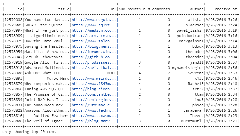
df = spark.read.csv("/sparkdata/Hacker_news.csv", header=True)
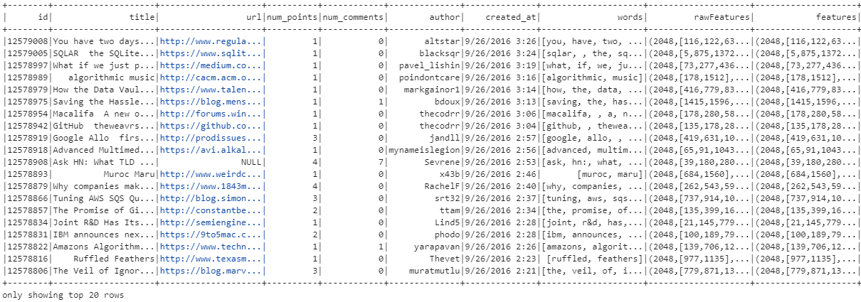
df.show()Firstly, we import the SparkSession class, which is the entry point to Spark functionality. Next, we import Tokenizer, HashingTF, IDF, MinHashLSH features, these are the necessary classes for text processing and similarity calculation. And lastly, we require col, rand, collect_list, struct, monotonically_increasing_id which perform various functions needed for DataFrame operations.
SparkSession is initialized and the dataset of Hacker News articles from a CSV file is loaded into a DataFrame. This DataFrame represents the dataset, with each row corresponding to a news article and each column containing different attributes such as the article's title, URL, ID, author, etc.
The show() function is then called to display a preview of the loaded data, allowing users to inspect its structure and contents. This step is crucial for understanding the dataset's format and ensuring it was loaded correctly before proceeding with further analysis.
Output:
Tokenization of the 'title' column
# Tokenize the text
tokenizer = Tokenizer(inputCol="title", outputCol="words")
wordsData = tokenizer.transform(df)
wordsData.show()
Let us now continue to the stage where the text of each news article's title is tokenized, where we essentially split the text into individual words or tokens.
The Tokenizer class from PySpark's ML library is used for this purpose. It takes an input column (inputCol) containing the text to be tokenized, which in this case is the "title" column df and the output being stored in a new column named "words", specified by the outputCol parameter.
After defining the tokenizer, the transform method is called on the DataFrame df with the tokenizer object as an argument. This applies the tokenization process to each row, creating a new DataFrame called wordsData with an additional column named "words" containing the tokenized versions of the article titles.
This representation allows for easy manipulation and analysis of the tokenized text data and is a common preprocessing step in natural language processing (NLP) tasks.
Output:
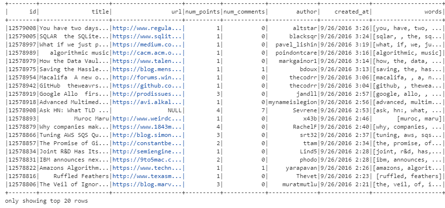
words has the title split into an array of strings!Creating feature vectors
# HashingTF to create feature vectors
hashingTF = HashingTF(inputCol="words", outputCol="rawFeatures", numFeatures=2048)
featurizedData = hashingTF.transform(wordsData)

# Cache the data
featurizedData.cache()

featurizedData.show()
Moving on, let us now apply the HashingTF transformation and caching operation on the tokenized data. HashingTF(Hashing Term Frequency) is a technique used to convert a collection of words into a fixed-size feature vector.
Here, the input for HashingTF is the "words" column generated by the Tokenizer, which splits the text into individual words. The output of the HashingTF transformation is stored in the "rawFeatures" column which contains the computed feature vectors representing the frequency of words in each article. The numFeatures=2048 parameter specifies the number of features (or dimensions) in the output feature vector. It determines the size of the hash space into which the words are hashed.
Additionally, after applying the HashingTF transformation, the resulting DataFrame, featurizedData is cached using the cache() function. Caching is a performance optimization technique that stores the DataFrame in memory or disk for faster access in subsequent operations to avoid expensive computation involved in generating the feature vectors when the data is reused multiple times in subsequent computations.
Output:
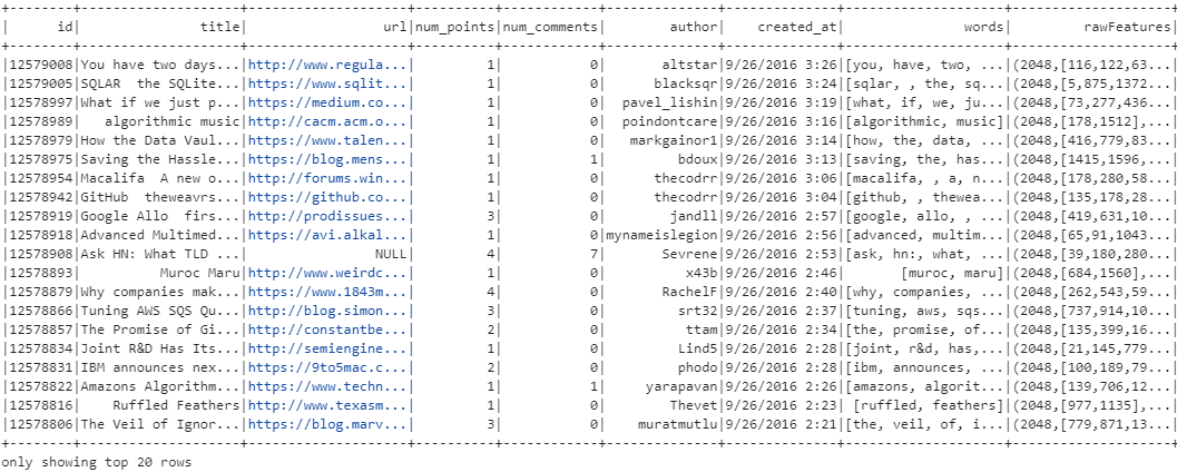
The representation of rawFeatures "(2048, [number1, number2,...])" indicates that the feature vector has a length of 2048 elements, with non-zero values at specific indices. In this format:
- "2048" denotes the total number of features or dimensions in the vector.
- "[number1, number2,...]" represents the indices of the non-zero elements in the vector, along with their corresponding values.
Since the feature vectors are generated using the HashingTF transformation, each word in the tokenized text is hashed to a specific index in the feature vector space. The non-zero values at these indices indicate the presence of the corresponding words in the text.
Feature Vector Transformation using IDF
# Fit the IDF model and transform the original feature vectors
idf = IDF(inputCol="rawFeatures", outputCol="features")
idfModel = idf.fit(featurizedData)
rescaledData = idfModel.transform(featurizedData)
rescaledData.show()
Continuing further, an IDF (Inverse Document Frequency) model is trained and applied to transform the original feature vectors.
The IDF model requires two parameters:
inputCol: The name of the input column containing the raw feature vectors. In our case, it is specified as"rawFeatures".outputCol: The name of the output column where the transformed feature vectors will be stored. Here, it is specified as"features".
After initializing the IDF model with these parameters, it is fitted to the featurizedData DataFrame using the fit() method for computing IDF weights for each term in the dataset based on the raw feature vectors and the transform() method is applied to the featurizedData DataFrame using the trained IDF model (idfModel) to compute the IDF-transformed feature vectors and store them in the specified output column "features".
Output:
We use IDF to weigh the importance of words in the dataset relative to a corpus of all other words. The IDF value increases proportionally to the number of documents in the corpus that do not contain the word, which helps in identifying words that are unique or rare across the dataset. This is important because common words like "the", "is", etc., may appear frequently in many documents but may not carry significant meaning in distinguishing one document from another.
Using MinHashLSH Model for Approximate Similarity Search
# Create and fit the MinHashLSH model to the feature vectors
mh = MinHashLSH(inputCol="features", outputCol="hashes", numHashTables=5)
model = mh.fit(rescaledData)

# Transform the feature data to include hash values
transformedData = model.transform(rescaledData)
transformedData.show()
We move on to creating and applying a MinHashLSH (MinHash Locality Sensitive Hashing) model on the feature vectors. which is used for approximate similarity search which works by transforming high-dimensional feature vectors into a set of hash values, where similar vectors are likely to have similar hash values.
First, we initialize the MinHashLSH model (mh) with parameters such as the input column (inputCol) specifying the feature vectors to be hashed, the output column (outputCol) where the hash values will be stored and the number of hash tables (numHashTables) to use.
Next, we fit the MinHashLSH model to the feature vectors represented by the DataFrame rescaledData. This process involves computing MinHash signatures for each feature vector and constructing hash tables based on these signatures. and the result is stored in the variable model.
Finally, we apply the trained MinHashLSH model to the rescaledData DataFrame using the transform() method. This operation transforms the feature data to include hash values, and the resulting DataFrame transformedData contains the original feature vectors along with their corresponding hash values in the specified output column "hashes".
Output:
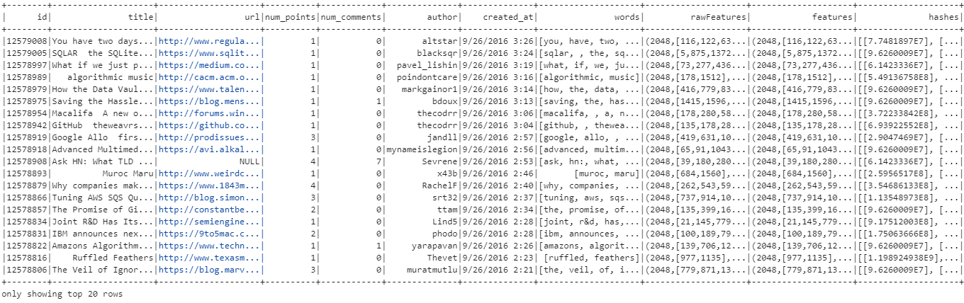
The "hashes" column represents the MinHash signatures generated for each feature vector using the MinHashLSH algorithm. Each element in the "hashes" column is an array containing numerical values, which are the hash signatures computed to efficiently approximate similarity between feature vectors.
Using approxSimilarityJoin for collecting similar news
# Randomly select 10 different news articles
sampledData = transformedData.orderBy(rand()).limit(10)

# Join the sampled data with the original set to find the top 10 similar articles for each
similarNews = model.approxSimilarityJoin(transformedData, sampledData, 0.81, distCol="JaccardDistance") \
    .select(
        col("datasetA.id").alias("idA"),
        col("datasetA.title").alias("titleA"),
        col("datasetB.id").alias("idB"),
        col("datasetB.title").alias("titleB"),
        col("JaccardDistance")
    ) \
    .filter("idA != idB") \

# Window definition for ordering within each group
windowSpec = Window.partitionBy("idB").orderBy("JaccardDistance")

# Order by distance within each group and assign row numbers
similarNews = similarNews.withColumn("row_num", row_number().over(windowSpec))

# Filter to keep only the top 10 similar news items for each group
similarNews = similarNews.filter(col("row_num") <= 10) \
    .orderBy("idB", "row_num") \
    .groupBy("idB", "titleB") \
    .agg(collect_list(struct(col("idA"), col("titleA"), col("JaccardDistance"))).alias("similarNews"))
- We have now reached the stage where we randomly select 10 different news articles from
transformedDatadone by ordering it randomly using therand()function and then limiting the result to 10 rows. - Approximate Similarity Join: Next, we use
approxSimilarityJoinfunction to perform an approximate similarity join between thetransformedDataDataFrame and thesampledDataDataFrame. It calculates the Jaccard distance between feature vectors and filters pairs with a distance less than or equal to 0.81. After the join operation, the result is selected with specific columns renamed for clarity using theselectfunction. - A window specification
windowSpecis defined to partition by the ID of the second article (idB) and order the rows within each partition by the Jaccard distance. Therow_numberfunction is used within each partition to assign a sequential row number to each row based on the ordering specified in the window. - Rows with row numbers greater than 10 are filtered out, ensuring only the top 10 similar news items for each article are retained. Finally, we perform Grouping and Aggregation, where the DataFrame is then grouped by the ID and title of the second article (
idBandtitleB) and aggregated usingcollect_listto gather the top 10 similar articles for each group.
Displaying the top 10 most similar news
import pandas as pd

# Convert DataFrame to Pandas DataFrame for better printing
similar_news_df = similarNews.toPandas()

# Output the similar news articles for the sampled news items
for _, row in similar_news_df.iterrows():
    print(f"\nTop 10 similar news articles for \"{row['titleB']}\":")
    for similar in row['similarNews']:
        print(f"- \"{similar['titleA']}\" (ID: {similar['idA']}, Jaccard Distance: {similar['JaccardDistance']})")

# Stop the Spark session
spark.stop()
We are almost ready! We firstly import the pandas library, we do this to convert similarNews into a Pandas DataFrame similar_news_df for better printing and manipulation capabilities. Then, it iterates over each row of the Pandas DataFrame and prints the top 10 similar news articles for each sampled news item.
The conversion to a Pandas DataFrame allows for more convenient printing using the iterrows() function to iterate over rows and access column values easily.
We conclude by stopping the Spark session to release resources and terminate the Spark application!
Output:
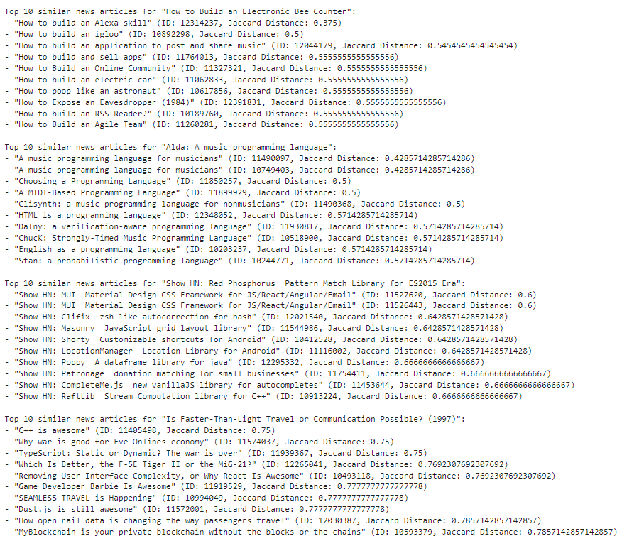
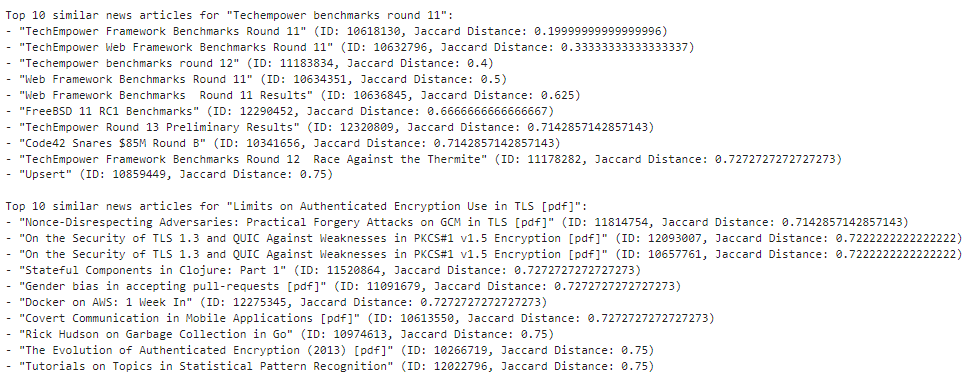
Out of the random 10 news articles that were chosen, the top 10 similar news articles related to each of them are as follows:
The first 4 of them are shown below:
The next 4 news articles:
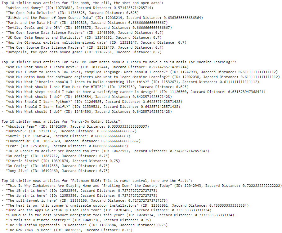
The 9th and the 10th news articles look like this:
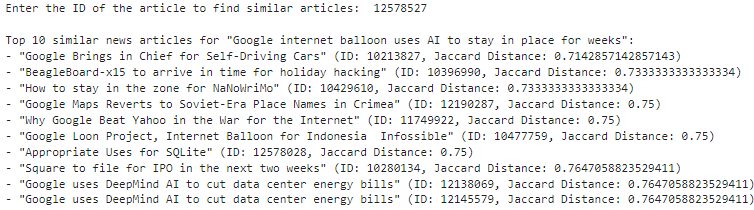
We can easily modify the code in such a manner that the user can enter a particular news id of their own and can easily obtain the top 10 most similar news articles for the id they've chosen!
# Transform the feature data to include hash values
transformedData = model.transform(rescaledData)

#MODIFICATION BEGINS HERE

article_id = input("Enter the ID of the article to find similar articles: ")
sampledData = transformedData.filter(col("id") == article_id)

#MODIFICATION ENDS HERE


#REST OF THE CODE REMAINS THE SAME
similarNews = model.approxSimilarityJoin(transformedData, sampledData, 0.81, distCol="JaccardDistance") \
    .select(
        col("datasetA.id").alias("idA"),
        col("datasetA.title").alias("titleA"),
        col("datasetB.id").alias("idB"),
        col("datasetB.title").alias("titleB"),
        col("JaccardDistance")
    ) \
    .filter("idA != idB") \

# Window definition for ordering within each group
windowSpec = Window.partitionBy("idB").orderBy("JaccardDistance")

# Order by distance within each group and assign row numbers
similarNews = similarNews.withColumn("row_num", row_number().over(windowSpec))

# Filter to keep only the top 10 similar news items for each group
similarNews = similarNews.filter(col("row_num") <= 10) \
    .orderBy("idB", "row_num") \
    .groupBy("idB", "titleB") \
    .agg(collect_list(struct(col("idA"), col("titleA"), col("JaccardDistance"))).alias("similarNews"))
Output:

The user is asked to input the id of their choice from the dataset and the results are displayed as shown below:
How can we obtain improved results?
In this section, we are exploring some key strategies for improving the outcomes of news article similarity analysis in PySpark. By adjusting parameters, one can refine their analyses to better capture nuanced similarities and deliver more relevant insights. Let's delve into these strategies and explore how they can be applied to enhance the effectiveness of news article similarity analysis.
There are a number of ways in which we can achieve this:
- Number of Features (HashingTF):
Adjusting the number of features parameter in the HashingTF stage allows us to control the dimensionality of the feature space. Increasing this parameter can capture more unique terms but may lead to higher computational overhead. For instance, upon increasing the value from 2048 to 4096, we can notice improved discrimination between articles, particularly in capturing finer semantic similarities.
- Number of Hash Tables (MinHashLSH):
The numHashTables parameter in the MinHashLSH stage determines the number of hash tables used for approximate nearest neighbor search. Higher values reduce false negatives but may impact performance.
An example: With a dataset featuring 4096 features, a good metric would be to set the numHashTables value to the square root of the feature count (64 in our case) which would provide a more finely grained LSH structure. This results in more accurate similarity calculations without sacrificing performance significantly.
- Jaccard Distance Threshold:
The Jaccard distance threshold defines the minimum similarity required for articles to be considered relevant. Lowering this threshold captures more nuanced similarities but may also include more false positives.
Let us take a case where we initially set the Jaccard distance threshold to 0.8, filtering out articles with less than 80% similarity. However, by reducing the threshold to 0.7, we can observe a broader but more relevant set of similar articles, enhancing the analysis's granularity.
By iteratively adjusting these parameters and observing their effects on the similarity analysis results, we can fine-tune the algorithm to better suit our specific use case, ultimately enhancing the quality!
Conclusion
We hope that this would have provided you guys a good hands-on-experience on leveraging PySpark for news article similarity analysis. One can gain valuable insights into how similar news articles can be identified and analyzed at scale. PySpark's robust capabilities for data processing makes it an invaluable tool for text mining and recommendation systems in various industries.

By subscribing to our newsletter, you can stay updated on the latest developments in data science, machine learning and so on, ensuring you remain at the forefront of innovation in this amazing field. Don't miss out on future insights and tutorials in the world of AI – subscribe today!


