Unlocking the Power of PySpark SQL: An end-to-end tutorial on App Store data

In the realm of data science and analytics, proficiency in handling vast datasets efficiently is paramount. Apache Spark has emerged as a cornerstone technology for scalable and high-performance data processing. Pairing Spark with Python, through PySpark, it offers a great combination for data professionals to tackle diverse analytical challenges.

It is essential to know how to effectively evaluate large amounts of data in today's data-driven society. We'll take you from the fundamentals of PySpark SQL to more complex methods and prcoessing through this blog. This tutorial will provide you the tools you need to confidently take on real-world data challenges. Together, let's explore PySpark SQL's capabilities!

• We'll begin by exploring the setup process for a PySpark Notebook using Docker.
• Following that, we'll delve into essential SQL operations, including select queries, group by, and order by statements.
• Our journey will then progress to a comprehensive overview of functions, encompassing aggregate, scalar, and window functions.
• Finally, we'll conclude with a discussion on the utility and implementation of User Defined Functions (UDFs).

Setting up the PySpark Notebook using Docker

Step 1: Pulling the all-spark-notebook Image

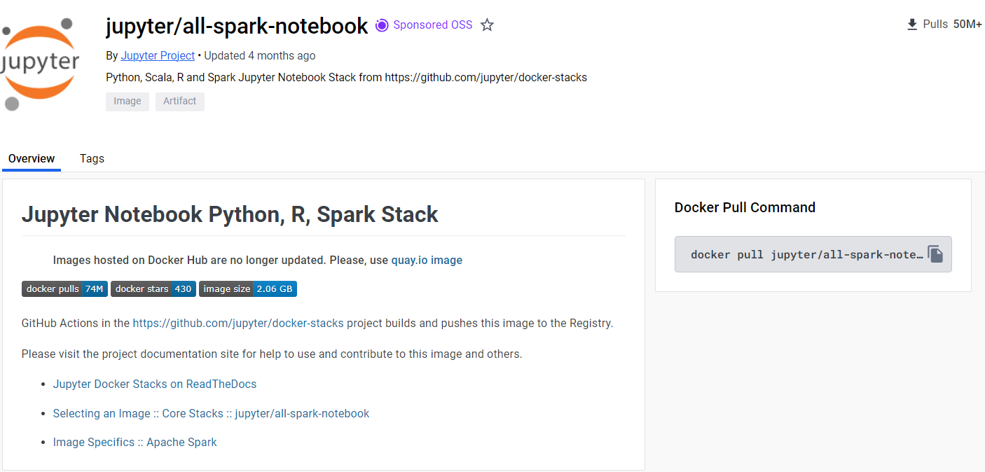
Let us start by visiting the Docker Hub page from where can pull the Spark Notebook image ( click here ). Now, let us pull the jupyter/all-spark-notebook image, which is packed with Spark 3.5.0 with the following command on your command prompt/terminal :

docker pull jupyter/all-spark-notebook:spark-3.5.0

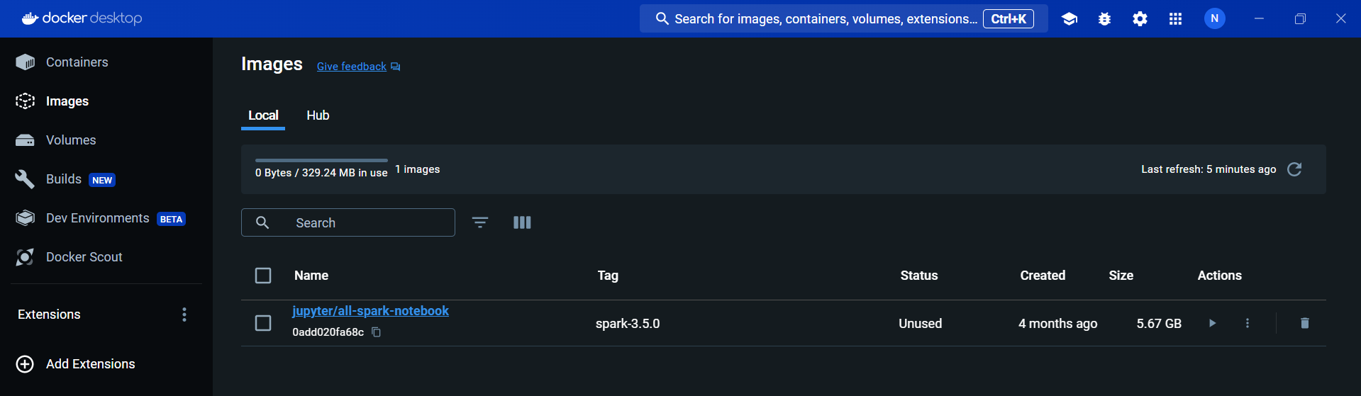
Once it's done, on your Docker Desktop, you can see that the notebook image is displayed on the Images module, which confirms the successful procedure carried out.

Step 2: Set Up Your Workspace

Before we run our Docker image, we need to set up a directory/folder where our dataset will be stored.

Therefore, create a directory named sparkdata in your workspace. In this directory you can store your required data, in our case, we are storing a particular CSV file with which we'll be working today. This CSV file is a dataset that contains the stats of most applications on Play Store.

Check out the dataset below for download.

The same dataset can be accessed through this link. (click here)

Step 3: Run the Docker Image

Now, let's run the Docker image and map our sparkdata directory to the container.

Replace /Users/datasciencefm/workspace/sparkdata with the path to your sparkdata directory.

docker run -d -P --name notebook -v C:\Users\datasciencefm\workspace\sparkdata:/sparkdata  jupyter/all-spark-notebook:spark-3.5.0

Docker: error while creating mount source path. How can i fix it?

Tks all, idk why, but now its working I am learning to use docker. I am trying to mount a host directory in a Docker container: >docker run -it -v /Users/Kell/Desktop/data:/home/data 77 And th…

Stack Overflowkell

Step 4: Retrieve the Port Mapping

When we run a service inside a Docker container, it's isolated from the host system. To interact with services running inside the container, we need to map the container's ports to ports on the host system.

To access the Jupyter Notebook, we need to know which host port has been mapped to the container's port 8888. To get the value of the host port, execute the following command:

docker port notebook 8888

For us, the output was 0.0.0.0:32768.

This indicates that the Jupyter Notebook service running inside the container's port 8888 is mapped to the host system's port 32768. This means that to access the Jupyter Notebook from the host system, we would use the host's IP address followed by port 32768.

Step 5: Fetch the Notebook Token

Jupyter Notebooks are secured by tokens to prevent unauthorized access. To obtain this token, we use the command :

docker logs --tail 3 notebook

This command retrieves the last three lines of log output from the Docker container named notebook, where our Jupyter Notebook service is running.

The output of this command will include URLs, and the second URL usually resembles http://127.0.0.1:8888/lab?token=YOUR_TOKEN_HERE. YOUR_TOKEN_HERE is a placeholder for the actual token.

For us, the token was http://127.0.0.1:8888/lab?token=a22226f11ace778a3589d4ec880359d03a10c0b21572d984

This token needs to be appended to the end of the URL when accessing the Jupyter Notebook, ensuring that only users with the correct token can access the notebook.

Step 6: Access the Jupyter Notebook

Replace the default port in the URL with the host port one you identified in Step 4(which was 32768 for us). In our case, the updated URL is:

http://127.0.0.1:32768/lab?token=a22226f11ace778a3589d4ec880359d03a10c0b21572d984

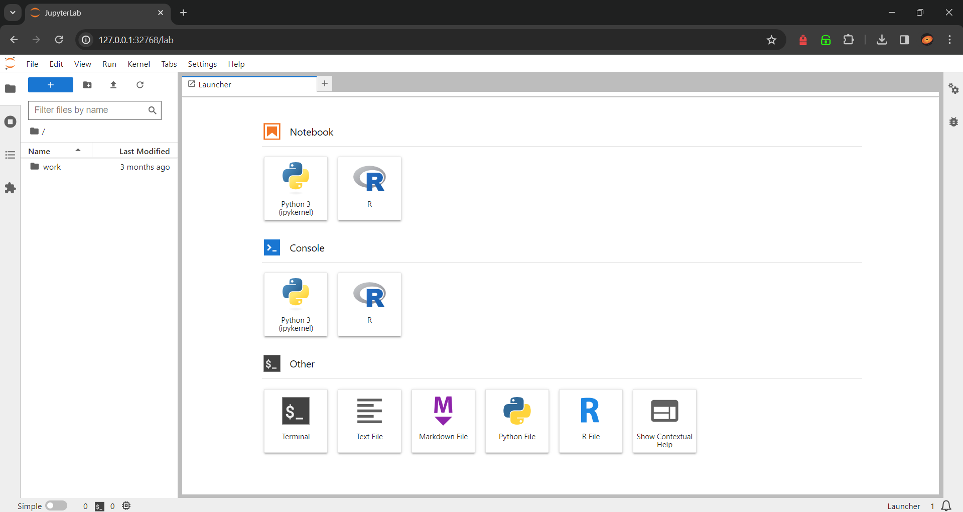
Simply paste this URL into your browser to open your Jupyter Notebook! And your setup is now ready!

Applying queries to the real-life Android Apps dataset

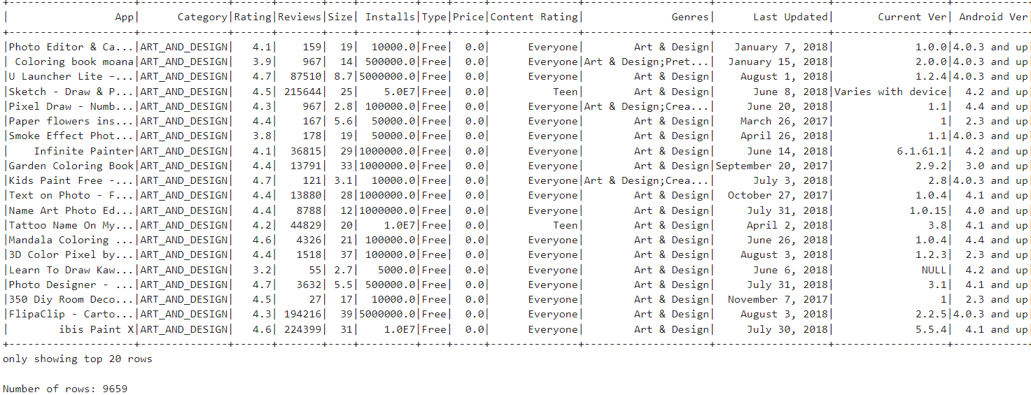
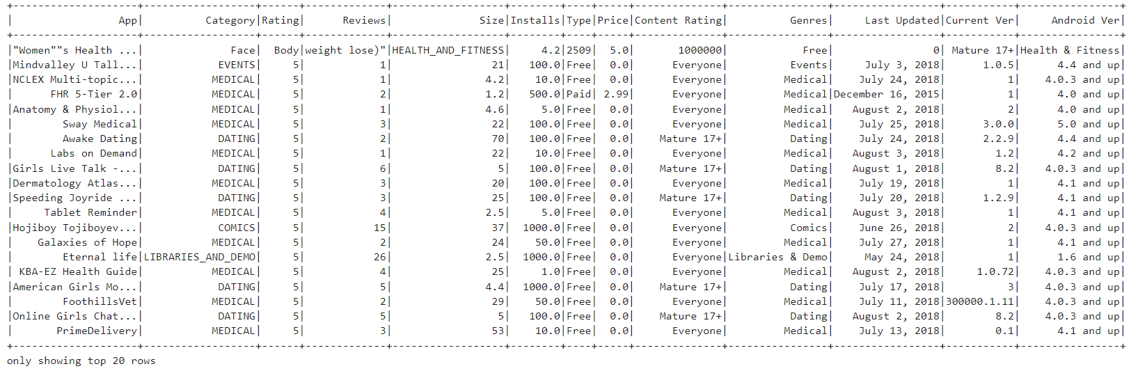
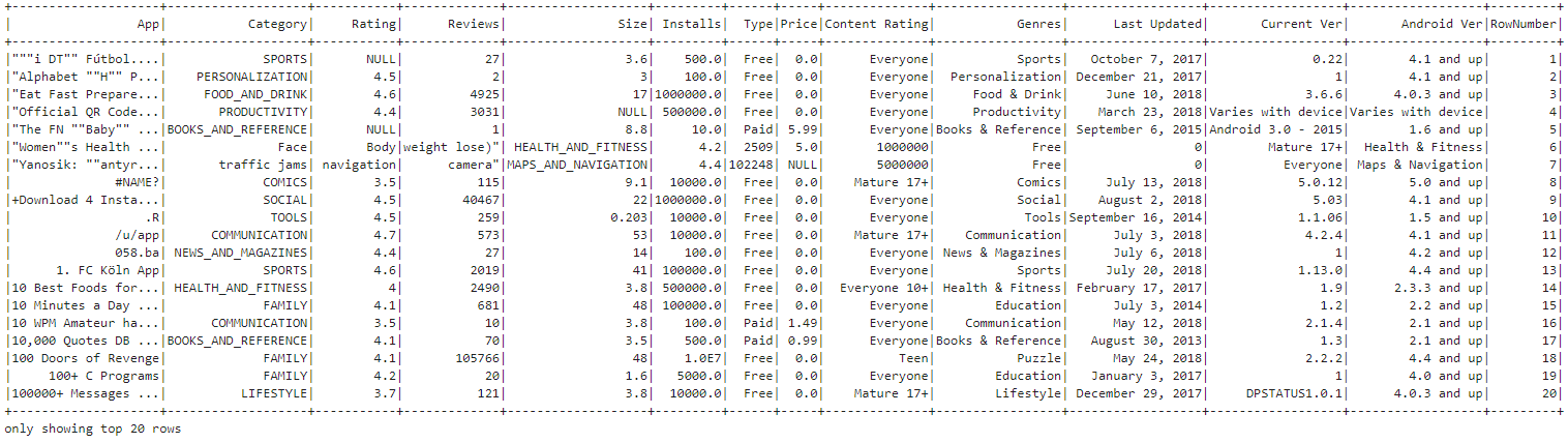
Once you open the Notebook, you can start exploring the Android Apps dataset by writing and executing code in cells. Let's start by looking at the first 20 rows of our dataset to get a quick overview of its contents.

from pyspark.sql import SparkSession

# Spark session & context
spark = SparkSession.builder.master("local").getOrCreate()
sc = spark.sparkContext

# Reading CSV file from /sparkdata folder
csv_path = "/sparkdata/androidapps.csv"  # This will read any CSV file in the /sparkdata folder
df = spark.read.csv(csv_path, header=True, inferSchema=True)  # Assuming the CSV has a header

# Show the DataFrame
df.show()

# If you want to perform any action on DataFrame
# For instance, to get the count of rows:
print("Number of rows:", df.count())

# Create a temporary view to query the DataFrame using SQL
df.createOrReplaceTempView("androidapps")

In this code, the SparkSession and SparkContext are created to interact with Apache Spark. The SparkSession (spark) serves as the entry point for Spark functionality, meanwhile, the SparkContext (sc) manages the execution of Spark tasks and resources, particularly for lower-level operations. Together, they enable data processing tasks, such as reading a CSV file (spark.read.csv), displaying DataFrame contents (df.show()), and creating a temporary view (df.createOrReplaceTempView) for querying using SQL syntax.

Output:

Since we now know how our data frame looks like, let us get our hands dirty with some queries! We shall start with something simple and progressively move on to more complex problems.

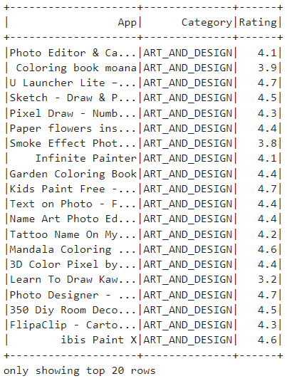
Query 1: Let us see how to display only the particular columns that we prefer using the following code:

# Selecting specific columns 'App', 'Category', and 'Rating'
selected_columns_df = df.select('App', 'Category', 'Rating')

# Show the resulting DataFrame
selected_columns_df.show()

Using the select keyword, specific columns 'App', 'Category', and 'Rating' from the DataFrame df are displayed.

Output:

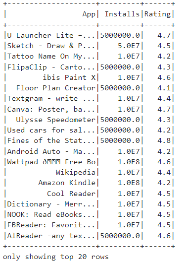
Query 2: Now, let us list the apps with more than 1 million installs and a rating higher than 4 in the dataset.

from pyspark.sql.functions import col

# Applying filter conditions using DataFrame functions
query_result = df.select('App', 'Installs', 'Rating') \
    .filter((col('Installs') > 1000000) & (col('Rating') > 4.0))

# Show the query result
query_result.show()

In this code, we have filtered(using the filter keyword) the DataFrame rows based on two conditions: 'Installs' greater than 1,000,000 and 'Rating' greater than 4.0. & is a conditional operator combines two conditions and evaluates to true only if both conditions are true simultaneously. Both conditions must be met for a row to be included in the query result!

Output:

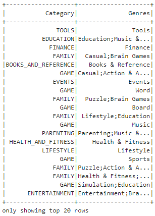
Query 3: Next, we shall show the distinct categories and genres in our dataset.

# Selecting distinct values from the 'Category' and 'Genres' columns
distinct_categories_genres_df = df.select('Category', 'Genres').distinct()

# Show the distinct categories and genres
distinct_categories_genres_df.show()

This code uses distinct keyword, which selects unique combinations of values from the 'Category' and 'Genres' columns in the DataFrame and displays them.

Output:

GROUP BY and ORDER BY queries

 A GROUP BY statement sorts data by grouping it based on column(s) you specify in the query, it is mostly used with aggregate functions. An ORDER BY allows you to organize result sets alphabetically or numerically and in ascending or descending order

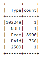
Query 4: Let us perform grouping on the 'Type' column and get the total number of free and paid apps in the dataset.

# Simple group by 'Type' and count the number of apps in each type
type_counts_df = df.groupBy('Type').count()

# Show the resulting DataFrame
type_counts_df.show()

This code performs a simple group by operation on the 'Type' column and counts the number of apps in each type, we use it with count aggregate function, which we'll know more about soon!

Output:

Query 5: We need to obtain the top rated apps in the dataset.

from pyspark.sql.functions import desc

# Simple order by 'Rating' in descending order
sorted_apps_df = df.orderBy(desc('Rating'))

# Show the resulting DataFrame
sorted_apps_df.show()

The code orders the DataFrame by a particular column called the 'Rating' column in descending order, resulting in the apps sorted based on their ratings from highest to lowest.

Output:

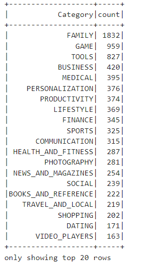
Query 6: Let us obtain the the number of apps in each category in decreasing manner.

# Group by 'Category' and calculate the count of apps in each category, then order by the count in descending order
category_counts_df = df.groupBy('Category').count().orderBy(desc('count'))

# Show the resulting DataFrame
category_counts_df.show()

We group by the 'Category' column to calculate the count of apps in each category. Secondly, we order the result by the count in descending order, showing the categories with the highest number of apps first.

Output:

Functions

Aggregate Functions

Aggregate functions are used to perform calculations on groups of data within a DataFrame. These functions summarize or compute statistics on a dataset, such as finding the sum, count, average, minimum, or maximum value of a column. They are essential for summarizing and analyzing large datasets efficiently.

Query 7: Calculating the total number of installs.

from pyspark.sql.functions import sum

# Calculate the total number of installs
total_installs = df.select(sum('Installs')).collect()[0][0]
print("Total number of installs:", total_installs)

We obtain the total number of installs across all apps in the DataFrame by applying the sum aggregate function to the 'Installs' column.

Output:

Query 8: Finding the average rating of all apps.

from pyspark.sql.functions import avg

# Find the average rating of all apps
average_rating = df.select(avg('Rating')).collect()[0][0]
print("Average rating of all apps:", average_rating)

Similar to the previous query, we use the average( avg) aggregate function.

Output:

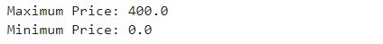
Query 9: Listing the maximum and minimum price values of the applications.

from pyspark.sql.functions import max, min

# Find the maximum and minimum values in the 'Price' column
max_price = df.select(max('Price')).collect()[0][0]
min_price = df.select(min('Price')).collect()[0][0]

print("Maximum Price:", max_price)
print("Minimum Price:", min_price)

We utilize the max and min aggregate functions to find the maximum and minimum values in the 'Price' column.

Output:

Moving onto slightly more complex queries,

Query 10: Calculating the category with the highest average rating.

from pyspark.sql.functions import avg

# Calculate the average rating for each category
avg_rating_df = df.groupBy('Category').agg(avg('Rating').alias('AvgRating'))

# Find the maximum average rating
max_avg_rating = avg_rating_df.select(max('AvgRating')).collect()[0][0]

# Find the category with the highest average rating
max_avg_rating_category = avg_rating_df.filter(avg_rating_df['AvgRating'] == max_avg_rating) \
                                     .select('Category').first()[0]

print("Category with the highest average rating:", max_avg_rating_category)

We firstly receive the average rating for each category using the avg aggregate function, then we identify the category with the highest average rating by finding the maximum average rating and filtering to retrieve the corresponding category.

Output:

Query 11: Let us calculate the category with the highest total number of installs.

from pyspark.sql.functions import sum, max

# Calculate the total number of installs for each category
total_installs_df = df.groupBy('Category').agg(sum('Installs').alias('TotalInstalls'))

# Find the maximum total number of installs
max_installs = total_installs_df.select(max('TotalInstalls')).collect()[0][0]

# Find the category with the highest total number of installs
max_installs_category = total_installs_df.filter(total_installs_df['TotalInstalls'] == max_installs) \
                                        .select('Category').first()[0]

print("Category with the highest total number of installs:", max_installs_category)

This code calculates the total number of installs for each category using the sum aggregate function, then identifies the category with the highest total number of installs by finding the maximum total installs.

Output:

Scalar Functions

Scalar functions operate on individual values within a DataFrame's columns, producing a single output value for each input value. These functions can be applied to manipulate, transform, or compute values within DataFrame columns on a row-by-row basis.

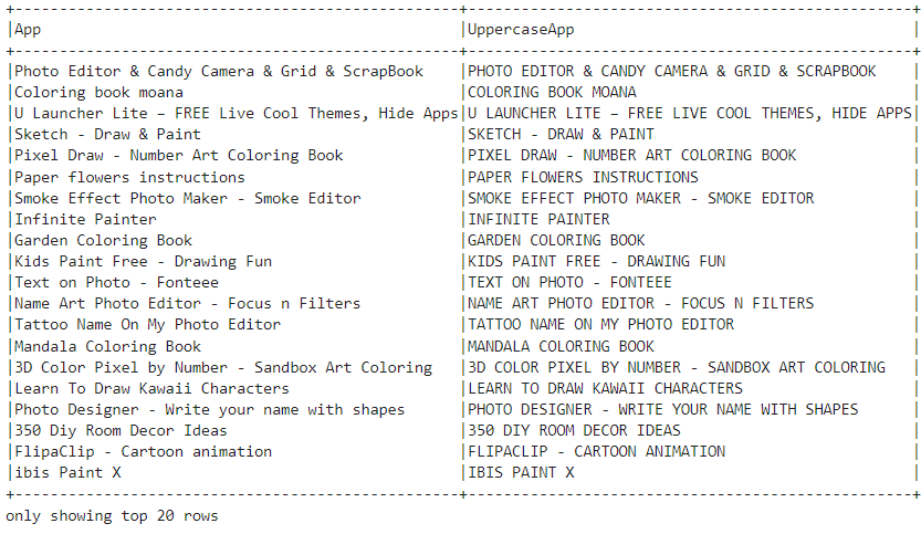
Query 12: Converting Application Names to Uppercase.

from pyspark.sql.functions import upper

# Convert the 'App' column values to uppercase
uppercase_apps_df = df.select('App', upper('App').alias('UppercaseApp'))

# Show the result
uppercase_apps_df.show(truncate=False)

This snippet utilizes the upper() scalar function to convert the values in the 'App' column of a DataFrame to uppercase, creating a new column named 'UppercaseApp', and displays the result.

Output:

Query 13: Concatenating Application Names with Their Genres.

from pyspark.sql.functions import concat

# Concatenate the 'App' and 'Genres' columns
concat_apps_df = df.select('App', 'Genres', concat('App', 'Genres').alias('AppWithGenres'))

# Show the result
concat_apps_df.show(truncate=False)

We employ the concat() scalar function to concatenate(join) the values in the 'App' and 'Genres' columns, creating a new column named 'AppWithGenres',

Output:

Window functions

Window functions are used to perform calculations across a group of rows that are related to the current row. One can calculate running totals, rankings and other analytical functions over a defined window of rows. These functions are typically used in conjunction with the Window specification, which defines the window frame over which the function operates, including the partitioning and ordering of rows within the frame.

Query 14: Assigning Row Number to Each Row.

from pyspark.sql.window import Window
from pyspark.sql.functions import row_number

# Define a window specification
window_spec = Window.orderBy('App')

# Assign a unique number to each row based on the order of the 'App' column
row_number_df = df.withColumn('RowNumber', row_number().over(window_spec))

# Show the result
row_number_df.show()

The window function in PySpark is used to assign a unique row number to each row of the DataFrame based on the order of the 'App' column, allowing for sequential numbering of rows without altering the original ordering. As we can see in the output, the last column contains the Row Number.

Output:

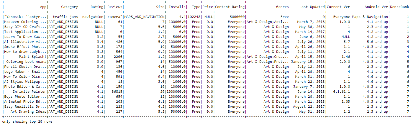
Query 15: Assignment of a dense Rank to each row based on Rating.

from pyspark.sql.functions import dense_rank

# Define a window specification
window_spec = Window.partitionBy('Category').orderBy('Rating')

# Assign a dense rank to each row within each category based on the 'Rating' column
dense_rank_df = df.withColumn('DenseRank', dense_rank().over(window_spec))

# Show the result
dense_rank_df.show()

We use a window function to assign a dense rank(that assigns consecutive integers to items with the same ranking order, without leaving gaps between ranks) to each row within each category based on the 'Rating' column, enabling the ranking of data within specific categories while maintaining the original ordering within each partition.

Output:

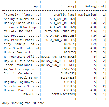
Query 16: Ranking each app in their category according to rating and displaying the top 3 apps in each category.

from pyspark.sql.window import Window
from pyspark.sql.functions import row_number, col

# Define a window specification partitioned by 'Category' and ordered by 'Rating' in descending order
window_spec = Window.partitionBy('Category').orderBy(col('Rating').desc())

# Use row_number() to assign a unique row number within each category based on the rating
ranked_apps_df = df.withColumn('Rank', row_number().over(window_spec))

# Filter only the top 3 apps within each category based on their rating
top_3_apps_df = ranked_apps_df.filter(col('Rank') <= 3)

# Show the result
top_3_apps_df.select('App', 'Category', 'Rating', 'Rank').show()

This code uses window functions to rank apps within each category by their rating in descending order, then filters to retain only the top 3 ranked apps in each category, displaying the results with their respective ranks.

Output:

User Defined Functions

User Defined Functions (UDFs) allow users to define custom functions to apply transformations or calculations to DataFrame columns. These functions can be written in Python and then registered to be used within Spark SQL queries. UDFs offer flexibility for performing complex operations that are not directly supported by built-in Spark functions.

Let us look at some UDFs on our dataset!

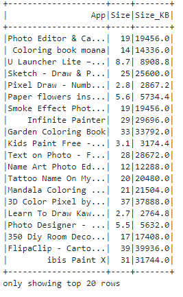
Query 17: Converting application size from MB to KB.

from pyspark.sql.types import FloatType
from pyspark.sql.functions import udf

# Define the UDF to convert size from MB to KB
def mb_to_kb(size_mb):
    try:
        return float(size_mb) * 1024.0
    except ValueError:
        return None

# Register the UDF
mb_to_kb_udf = udf(mb_to_kb, FloatType())

# Apply the UDF to the 'Size' column
android_apps_df = df.withColumn('Size_KB', mb_to_kb_udf('Size'))

# Show the result
android_apps_df.select('App', 'Size', 'Size_KB').show()

This code defines a User Defined Function (UDF) named mb_to_kb that converts size from megabytes (MB) to kilobytes (KB). The function takes a size in MB as input, converts it to KB, and returns the result. The UDF is registered using udf() function from PySpark, specifying the input and output types. Then, it's applied to the 'Size' column and lastly we create a new column named 'Size_KB', which is finally displayed.

Output:

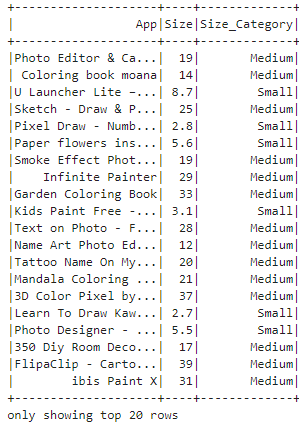
Query 18: Categorizing apps into small, medium or large.

from pyspark.sql.types import FloatType
from pyspark.sql.functions import udf

# Define the UDF to categorize apps by size
def categorize_size(size):
    try:
        size = float(size)  # Convert size to float
        if size <= 10:
            return 'Small'
        elif 10 < size <= 100:
            return 'Medium'
        else:
            return 'Large'
    except ValueError:
        return None  # Return None for non-numeric values

# Register the UDF
categorize_size_udf = udf(categorize_size)

# Apply the UDF to the 'Size' column
android_apps_df = df.withColumn('Size_Category', categorize_size_udf('Size'))

# Show the result
android_apps_df.select('App', 'Size', 'Size_Category').show()

We create a UDF named categorize_size that categorizes apps based on their size into three categories: 'Small', 'Medium', and 'Large'. The function takes the size of the app as input, converts it to float, and assigns the category based on predefined size thresholds. We create a new column named 'Size_Category' which holds the category and finally shown as follows:

Output:

Query 19: Extracting First Word from App Names

from pyspark.sql.functions import udf
from pyspark.sql.types import StringType

def extract_first_word(app_name):
    try:
        return app_name.split()[0]
    except IndexError:
        return None

# Register the UDF
extract_first_word_udf = udf(extract_first_word, StringType())

# Apply the UDF to the 'App' column
android_apps_df = df.withColumn('First_Word', extract_first_word_udf('App'))

# Show the result
android_apps_df.select('App', 'First_Word').show()

A UDF named extract_first_word is formulated that extracts the first word from each app name. The function takes the app name as input, splits it by whitespace, and returns the first word. We create the column named 'First_Word'. Finally, the DataFrame is displayed!

Output:

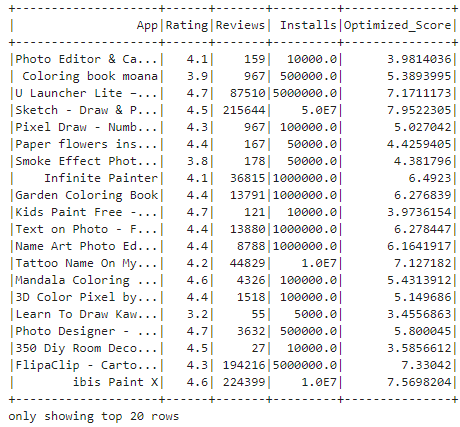
Query 20: Calculating "Optimized App Score", a hypothetical metric that indicates the overall performance or popularity of each application in the dataset.

from pyspark.sql.functions import udf
from pyspark.sql.types import FloatType
import math

# Define the UDF to calculate the optimized score
def calculate_optimized_score(rating, reviews, installs):
    try:
        # Convert installs and reviews to numeric values
        installs_numeric = int(installs)  # No need for replace() as installs is already numeric
        reviews_numeric = int(reviews)
        
        # Apply log transformation to reviews and installs to reduce skewness
        log_reviews = math.log1p(reviews_numeric)  # log1p is log(1+x) to handle 0 reviews gracefully
        log_installs = math.log1p(installs_numeric)
        
        # Normalize rating to be in a 0-1 range if it's not already (assuming 5 is the max rating)
        normalized_rating = float(rating) / 5
        
        # Assign weights to each component based on desired importance
        weight_rating = 0.5  # Example weight, adjust based on preference
        weight_reviews = 0.25
        weight_installs = 0.25
        
        # Calculate the weighted score
        score = (normalized_rating * weight_rating) + (log_reviews * weight_reviews) + (log_installs * weight_installs)
        return score
    except ValueError as e:
        # Handle cases where the data cannot be converted to numeric values
        print(f"Error processing input: {e}")
        return None

# Register the UDF with a FloatType return
optimized_score_udf = udf(calculate_optimized_score, FloatType())

# Apply the UDF to calculate the optimized score for each app
android_apps_df = df.withColumn('Optimized_Score', optimized_score_udf('Rating', 'Reviews', 'Installs'))

# Show the result
android_apps_df.select('App', 'Rating', 'Reviews', 'Installs', 'Optimized_Score').show()

calculate_optimized_score defines a user-defined function (UDF) to calculate an optimized score for Android apps based on their ratings, reviews, and installs. It applies logarithmic transformation to reviews and installs to reduce skewness and assigns weights to each component to adjust their influence on the final score. The UDF is then registered and applied to the DataFrame containing application data, resulting in the addition of an 'Optimized_Score' column. The result is finally shown.

Output:

Conclusion

Through this blog, I hope that each of you can gain an idea on how powerful this tool is, which can handle big data efficiently, unlocking insights and driving informed decision-making. Whether you're a data scientist, analyst or an engineer, learning to query and use PySpark for data analysis equips you with the skills to tackle real-world challenges in today's data-driven landscape.

Before you leave, do subscribe to our newsletter to get regular updates on all things happening in the universe of AI!

Stay tuned for more insightful blogs and tutorials, as we continue to explore the depths and applications in data science and analytics!