Analyze Chipotle orders dataset with Pandas to develop insights for digital ordering app
Pandas is a very powerful library enabling you to perform analytic operations with ease and speed. If you need to draw valid conclusions from your data, Pandas should be your first choice. In this series of posts, I'll show you how to use this feature-packed Python data analysis library.

Pandas is a very powerful library enabling you to perform analytic operations with ease and speed. If you need to draw valid conclusions from your data, Pandas should be your first choice. In this series of posts, I'll show you how to use this feature-packed Python data analysis library.
Imagine yourself to be a Data Analyst working for the restaurant chain Chipotle. You are given a dataset containing the details of the past 4000 orders. Your job is to analyze the data and find out what will help the chain make more optimal decisions regarding the development of a digital ordering system.
Your task is simple:
1) Find how much on average people spend per order.
2) Find the most typical combination of items in the orders.
3) Given a specific item, find out what has been ordered most frequently with it?
The data to download: https://raw.githubusercontent.com/justmarkham/DAT8/master/data/chipotle.tsv
Calculating the average value of an order
First of all we need to import the dataset into your python environment. To do so, we first need to import the necessary libraries.
import pandas as pd
import seaborn as sns
import matplotlib.pyplot as plt
import numpy as np
If you use a platform like Google Colab, you can connect your Google drive to it and store the data there. Otherwise you'll need to give Pandas the direct path to the file stored on your computer.
#Let's read in the data - our dataset is in the form of a tsv file. To read it in we use pd.read_csv but specify sep='\t'

chipotle = pd.read_csv('/content/drive/MyDrive/chipotle.tsv.txt', sep='\t')
After loading the data into the program, it's always good to take a quick look at the data, to check if everything is fine.
| index | order_id | quantity | item_name | choice_description | item_price |
|---|---|---|---|---|---|
| 0 | 1 | 1 | Chips and Fresh Tomato Salsa | NaN | $2.39 |
| 1 | 1 | 1 | Izze | [Clementine] | $3.39 |
| 2 | 1 | 1 | Nantucket Nectar | [Apple] | $3.39 |
| 3 | 1 | 1 | Chips and Tomatillo-Green Chili Salsa | NaN | $2.39 |
| 4 | 2 | 2 | Chicken Bowl | [Tomatillo-Red Chili Salsa (Hot), [Black Beans... | $16.98 |
| ... | ... | ... | ... | ... | ... |
| 4617 | 1833 | 1 | Steak Burrito | [Fresh Tomato Salsa, [Rice, Black Beans, Sour ... | $11.75 |
| 4618 | 1833 | 1 | Steak Burrito | [Fresh Tomato Salsa, [Rice, Sour Cream, Cheese... | $11.75 |
| 4619 | 1834 | 1 | Chicken Salad Bowl | [Fresh Tomato Salsa, [Fajita Vegetables, Pinto... | $11.25 |
| 4620 | 1834 | 1 | Chicken Salad Bowl | [Fresh Tomato Salsa, [Fajita Vegetables, Lettu... | $8.75 |
| 4621 | 1834 | 1 | Chicken Salad Bowl | [Fresh Tomato Salsa, [Fajita Vegetables, Pinto... | $8.75 |
Pre-processing the data
As you can see the column item_price has a $ in it. If we leave it like that Python will have a problem performing mathematical operations on the values. We need to remove the $ from the dataframe. The easiest way to do this is by using replace(). By specifying the argument inplace=True, we tell the function to change the values within our table. Otherwise, we'd get a copy of our dataframe with the values changed.
# For the sake of simplicity let's call our dataframe df
df = chipotle

df.iloc[:, 4].replace("\$", "", inplace=True, regex=True)

df| index | order_id | quantity | item_name | choice_description | item_price |
|---|---|---|---|---|---|
| 0 | 1 | 1 | Chips and Fresh Tomato Salsa | NaN | 2.39 |
| 1 | 1 | 1 | Izze | [Clementine] | 3.39 |
| 2 | 1 | 1 | Nantucket Nectar | [Apple] | 3.39 |
| 3 | 1 | 1 | Chips and Tomatillo-Green Chili Salsa | NaN | 2.39 |
| 4 | 2 | 2 | Chicken Bowl | [Tomatillo-Red Chili Salsa (Hot), [Black Beans... | 16.98 |
| ... | ... | ... | ... | ... | ... |
| 4617 | 1833 | 1 | Steak Burrito | [Fresh Tomato Salsa, [Rice, Black Beans, Sour ... | 11.75 |
| 4618 | 1833 | 1 | Steak Burrito | [Fresh Tomato Salsa, [Rice, Sour Cream, Cheese... | 11.75 |
| 4619 | 1834 | 1 | Chicken Salad Bowl | [Fresh Tomato Salsa, [Fajita Vegetables, Pinto... | 11.25 |
| 4620 | 1834 | 1 | Chicken Salad Bowl | [Fresh Tomato Salsa, [Fajita Vegetables, Lettu... | 8.75 |
| 4621 | 1834 | 1 | Chicken Salad Bowl | [Fresh Tomato Salsa, [Fajita Vegetables, Pinto... | 8.75 |
Another problem we face with this data is that price and quantity values are of types string, which means they are not treated as numbers. Try to multiply the quantity and item_price columns and you'll see that 2*2=22 not 4. This issue can be easily solved by changing the type of the values with pd.to_numeric() function. When we've done this we can multiply the price of ordered items by the quantity. We will store the result in a brand new column order_value. To add an extra column it's enough to call the dataframe name and add the name of the new column in square brackets.
item_price = pd.to_numeric(df['item_price'])

quantity = pd.to_numeric(df['quantity'])

df['order_value'] = quantity* item_price

df[:10]
To perform multiplication of all the values stored in each column, we first define new variables. Note that we convert the type of the values and get these variables with just one line of code.
| index | order_id | quantity | item_name | choice_description | item_price | order_value |
|---|---|---|---|---|---|---|
| 0 | 1 | 1 | Chips and Fresh Tomato Salsa | NaN | 2.39 | 2.39 |
| 1 | 1 | 1 | Izze | [Clementine] | 3.39 | 3.39 |
| 2 | 1 | 1 | Nantucket Nectar | [Apple] | 3.39 | 3.39 |
| 3 | 1 | 1 | Chips and Tomatillo-Green Chili Salsa | NaN | 2.39 | 2.39 |
| 4 | 2 | 2 | Chicken Bowl | [Tomatillo-Red Chili Salsa (Hot), [Black Beans... | 16.98 | 33.96 |
| 5 | 3 | 1 | Chicken Bowl | [Fresh Tomato Salsa (Mild), [Rice, Cheese, Sou... | 10.98 | 10.98 |
| 6 | 3 | 1 | Side of Chips | NaN | 1.69 | 1.69 |
| 7 | 4 | 1 | Steak Burrito | [Tomatillo Red Chili Salsa, [Fajita Vegetables... | 11.75 | 11.75 |
| 8 | 4 | 1 | Steak Soft Tacos | [Tomatillo Green Chili Salsa, [Pinto Beans, Ch... | 9.25 | 9.25 |
| 9 | 5 | 1 | Steak Burrito | [Fresh Tomato Salsa, [Rice, Black Beans, Pinto... | 9.25 | 9.25 |
Perhaps you noticed that each row in the table contains the data about a particular product that was ordered. Our task though, is to find how much an average order costs. Here comes another great Pandas function groupby(). We'll group the data based on the order_id and them sum up the prices per each product to get the full value of the order.
grouped = df.groupby(['order_id']).sum()
print(grouped)

order_id    quantity  order_value
1                4        11.56
2                2        33.96
3                2        12.67
4                2        21.00
5                2        13.70
...            ...          ...
1830             2        23.00
1831             3        12.90
1832             2        13.20
1833             2        23.50
1834             3        28.75
As you can see, after grouping the values per their order_id and adding up the values from all the rows with the same id we now have a new column with the full order value. It's now easy to calculate the average value.
Average vs. median
Yet, do I use average or median? That's a good question. Median price of the order simply means that half of the orders had bigger value and the second half of the orders smaller. Average and median can be similar but the average can be skewed by orders that were significantly more expensive or significantly cheaper so always make sure you understand their results.
To calculate the average and median in python, we'll use very simple functions. To calculate the average, we'll use mean(), and do calculate the median we'll use median().
grouped.mean()

quantity        2.711014
order_value    21.394231
grouped.median()
quantity 2.00
order_value 16.65
As you can see, these values are rather close, so it means that this dataset doesn't contain too many outliers.
General distribution of the order values
If we want to see what the distribution of the order values looks like, it's best to plot the data. To do so, we'll use the matplotlib and seaborn libraries.
plt.figure(figsize=(10,6))
sns.distplot(grouped)
plt.xlabel("Order Value")
plt.ylabel("Frequency")
plt.title("General Distribution of the Order Value", size=24)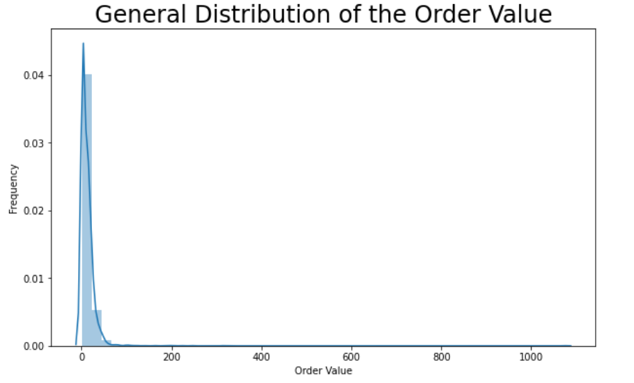
By the first look at this graph we can see that something's wrong. The vast majority of orders concentrates around $20-$30 but the plot reaches values up to $700. It suggests that we do have at least one outlier.
Let's use pandas sort_values() to see the highest order values.
sorted = df.sort_values('order_value', ascending=False)
print(sorted)

      order_id  quantity  ... item_price order_value
3598      1443        15  ...     44.25       663.75
4152      1660        10  ...     15.00       150.00
1254       511         4  ...     35.00       140.00
3602      1443         4  ...     35.00       140.00
3887      1559         8  ...     13.52       108.16
...        ...       ...  ...        ...         ...
107         47         1  ...      1.09         1.09
195         87         1  ...      1.09         1.09
434        188         1  ...      1.09         1.09
2814      1117         1  ...      1.09         1.09
4069      1629         1  ...      1.09         1.09
There's a huge gap between the first and second highest values. It's best if we get rid of this outlier to better visualize the data. We'll use drop() and specify the index of the value we want to get rid of.
data = df.drop([df.index[3598]])
data = data.groupby(['order_id']).sum()
Let's visualize the data again.
plt.figure(figsize=(10,6))
sns.distplot(data)
plt.xlabel("Order Value")
plt.ylabel("Frequency")
plt.title("General Distribution of the Order Value", size=24)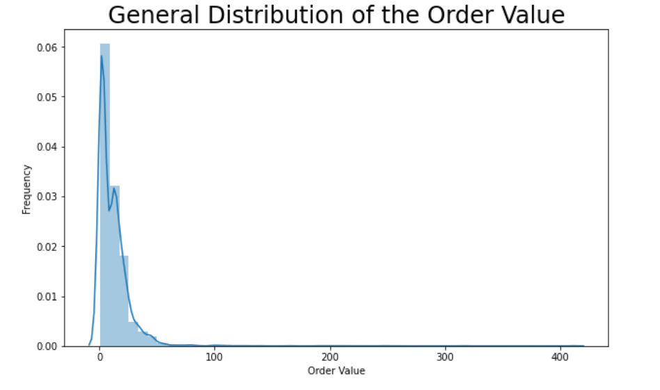
Much better, don't you think?
Finding the most common matches
So, now we know what the general distribution of orders looks like, we can move on to the second task. Let's find out what kind of products customers like to order together. If we have this knowledge, the Chipotle's management may decide to introduce a concept of meals.
To deal with this problem, we'll use pandas groupby() again. As I told you before Pandas is a super flexible library and using this simple function we'll know what we need in a second. We will group item_name per order_id and then use value_counts().
common_match = df.groupby('order_id')['item_name'].unique().astype(str).value_counts()
common_match[:6]

['Chicken Bowl' 'Chips and Guacamole']                  68
['Chicken Bowl']                                        61
['Chicken Burrito']                                     51
['Chicken Burrito' 'Chips and Guacamole']               37
['Steak Burrito' 'Chips and Guacamole']                 26
													    ...
['Steak Bowl' 'Canned Soft Drink' 'Chips and Guacamole'] 1
After looking at the results, we can see that Burrito and Bowl are the most common choices and they're usually matched with Chips. Sounds great! Drinks are ordered less often.
Finding the most common matches for each item
We know what the majority of people like to order, but let's dig deeper. Let's find out what people like to order with every other product in our menu. With this knowledge Chipotle could introduce online menu with the recommendations of the most popular choices .
Once again we'll use pandas groupby() and sort_values(), but this time slightly different.
df1 = df.reset_index()
df1 = df1.merge(df1, on='order_id').query('index_x > index_y')

df1 = pd.DataFrame(np.sort(df1[['item_name_x', 'item_name_y']].to_numpy(), axis=1))
df1.groupby([*df1]).size().sort_values(ascending=False)

Chicken Bowl         Chips and Guacamole    179
                     Chicken Bowl           164
                     Chicken Burrito        155
                     Chips                  143
Canned Soft Drink    Chicken Bowl           134
                                           ...
Barbacoa Salad Bowl  Canned Soft Drink        1
                     Bottled Water            1
                     Barbacoa Soft Tacos      1
Carnitas Bowl        Carnitas Bowl            1
Barbacoa Salad Bowl  Barbacoa Salad Bowl      1
The result shows us exactly what was bought with every item of the menu with its frequency.
Conclusions
We've managed to find the answer to each question put, and we can now share our conclusions with the management, together with the processed data for further analysis.
We found out that:
1) The majority of orders was of less than $20 value.
2) The most common meal of choice is Chicken Bowl with Chips.
3) We know exactly what people order with each product allowing us to build a simple recommender to show most frequently ordered items.