Leveraging AI for Financial Insights: From Data Fetching to Time Series Analysis
Performing financial analysis by automating data fetching, generating complex SQL queries and performing detailed time series analysis, turning raw financial data into actionable insights.

In today's fast-paced financial landscape, the collaboration between finance and AI is revolutionizing the way we analyze and interpret data, especially when it comes to capital markets. Therefore, it would be a fun expedition to explore how to leverage advanced AI tools for enhancing financial analysis.
Today's journey:
- We'll begin by harnessing the robust capabilities of the Yahoo Finance API to fetch real-time financial data.
- Next, we'll delve into the realm of intelligent automation, using LLMs to craft sophisticated SQL queries that streamline our data processing.
- Finally, we'll unveil the power of OpenAI's Assistant to perform intricate time series analysis, transforming raw data into actionable insights.
Join in as we uncover the connection between AI and finance, paving the way for smarter, data-driven decision-making.
Fetching data from Yahoo Finance API
Yahoo Finance is a widely-used platform that provides comprehensive financial information, including stock quotes, financial reports and market data. Utilizing the Yahoo Finance API allows for efficient and automated retrieval of this valuable data, making it an essential tool for investors, analysts and developers working on financial applications. In this section, we will explore how to access and fetch data from the Yahoo Finance API, providing a step-by-step guide to obtain and manipulate financial data accordingly. Whether you're tracking stock performance, analyzing market trends or conducting financial research, leveraging the Yahoo Finance API can significantly enhance your data acquisition and analysis capabilities.
Here's an example of how the data can be fetched:
We will first install the yfinance library using pip:
pip install yfinance
yfinance offers a large amount of financial data for free, here are a few examples shown below:
import yfinance as yf

msft = yf.Ticker("MSFT")

# get all stock info
msft.info

# get historical market data
hist = msft.history(period="1mo")

# show meta information about the history (requires history() to be called first)
msft.history_metadata

# show actions (dividends, splits, capital gains)
msft.actions
msft.dividends
msft.splits
msft.capital_gains  # only for mutual funds & etfs

# show share count
msft.get_shares_full(start="2024-01-01", end=None)

# show financials:
# - income statement
msft.income_stmt
msft.quarterly_income_stmt
# - balance sheet
msft.balance_sheet
msft.quarterly_balance_sheet
# - cash flow statement
msft.cashflow
msft.quarterly_cashflow

# show holders
msft.major_holders
msft.institutional_holders
msft.mutualfund_holders
msft.insider_transactions
msft.insider_purchases
msft.insider_roster_holders

# show recommendations
msft.recommendations
msft.recommendations_summary
msft.upgrades_downgrades


# show news
msft.news
To access more information, you can refer to the link below:
We'll focus on the feature to access stock data for multiple large-scale companies for the last 5 years. To do this, let us first store the data using SQL to a database for easy access.
This is how the schema looks like, we shall create a table called stock_data:
CREATE TABLE stock_data (
        date DATE,
        open FLOAT,
        high FLOAT,
        low FLOAT,
        close FLOAT,
        volume BIGINT,
        ticker TEXT
);date(DATE): The date of the stock data entry.open(FLOAT): The opening price of the stock on that date.high(FLOAT): The highest price of the stock on that date.low(FLOAT): The lowest price of the stock on that date.close(FLOAT): The closing price of the stock on that date.volume(BIGINT): The number of shares traded on that date.ticker(TEXT): The stock ticker symbol representing the company.
This table is designed to store daily stock market data for various companies.
To populate the database with stock info for the past 5 years:
import psycopg2
import yfinance as yf
import pandas as pd

# Database connection parameters
db_params = {
    'dbname': 'your_db_name',
    'user': 'your_username',
    'password': 'your_password',
    'host': 'your_host',
    'port': port_number
}

# Function to connect to the database
def connect_to_db(db_params):
    conn = psycopg2.connect(
        dbname=db_params['dbname'],
        user=db_params['user'],
        password=db_params['password'],
        host=db_params['host'],
        port=db_params['port']
    )
    return conn

# Function to download and format data for a single stock
def download_and_format_stock_data(ticker, start_date, end_date, retries=3):
    for i in range(retries):
        try:
            stock_data = yf.download(ticker, start=start_date, end=end_date)
            if not stock_data.empty:
                stock_data.reset_index(inplace=True)
                stock_data['ticker'] = ticker
                stock_data = stock_data[['Date', 'Open', 'High', 'Low', 'Close', 'Volume', 'ticker']]
                stock_data.columns = ['date', 'open', 'high', 'low', 'close', 'volume', 'ticker']
                return stock_data
        except Exception as e:
            print(f"Attempt {i+1} failed for {ticker}: {e}")
    return pd.DataFrame()

# Function to insert data into the stock_data table
def insert_data(conn, stock_data):
    insert_query = '''
    INSERT INTO stock_data (date, open, high, low, close, volume, ticker)
    VALUES (%s, %s, %s, %s, %s, %s, %s)
    '''
    with conn.cursor() as cursor:
        for _, row in stock_data.iterrows():
            cursor.execute(insert_query, tuple(row))
        conn.commit()

# Define the list of stock tickers and the time period
tickers = [
    'AAPL', 'MSFT', 'GOOGL', 'AMZN', 'TSLA', 'META', 'NVDA', 'NFLX', 'INTC', 'AMD',
    'IBM', 'ORCL', 'CSCO', 'ADBE', 'PYPL', 'QCOM', 'TXN', 'AVGO', 'CRM', 'SAP'
]
start_date = '2019-07-18'
end_date = '2024-07-18'

# Main function to execute the process
def main():
    conn = connect_to_db(db_params)

    for ticker in tickers:
        print(f"Processing {ticker}...")
        stock_data = download_and_format_stock_data(ticker, start_date, end_date)
        if not stock_data.empty:
            insert_data(conn, stock_data)
        else:
            print(f"No data found for {ticker}")

    conn.close()

if __name__ == "__main__":
    main()
- Imports and Setup: Imports
psycopg2,yfinance, andpandas. Defines database connection parameters. - Database Connection:
connect_to_db()function establishes a connection to the PostgreSQL database. - Download Stock Data:
download_and_format_stock_data()function fetches stock data for a given ticker and date range, retries up to 3 times if necessary, formats the data, and returns it. - Insert Data:
insert_data()function inserts the formatted stock data into thestock_datatable in the database. - Main Execution: The
main()function connects to the database, processes each ticker by downloading and inserting data, and closes the connection.
Generating SQL queries using GPT-4-Turbo for our data
We will utilize the text-to-SQL approach with GPT-4-Turbo to convert natural language queries into SQL statements. These generated SQL queries will then be executed to retrieve and inspect the output from our database.
from openai import OpenAI
OPENAI_API_KEY = 'ENTER_YOUR_API_KEY'

# Initialize the OpenAI client with your API key
client = OpenAI(api_key=OPENAI_API_KEY)


response = client.chat.completions.create(
  model="gpt-4-turbo",
  messages=[
    {"role": "system", "content": """ You are an expert in generating SQL queries, particularly for PostgreSQL databases.
     Instructions:
     1. When provided with an input question in natural language, your task is to generate a syntactically correct SQL query that can be executed
      on a PostgreSQL database.
     2. Your responses should only include the SQL query without any explanations or assumptions.
     3. Ensure that the SQL queries you generate are efficient and follow best practices for PostgreSQL.
     4. Avoid statements like 'Based on the context, ...' or 'The context information ...' or anything along those lines. DO NOT include any additional information.

     The schema looks like this:
     Table: stock_data
     Columns:   date DATE,
        open FLOAT,
        high FLOAT,
        low FLOAT,
        close FLOAT,
        volume BIGINT,
        ticker TEXT
    );
     """},
    {"role": "user", "content": """

      User Query: 'Enter your user query here'

     """

   }
  ]
)

print(response.choices[0].message.content)- Role prompting: "You are an expert in generating SQL queries, particularly for PostgreSQL databases."
- Establishes GPT-4-Turbo's role as a specialized expert, focusing the model's responses on generating accurate SQL queries for PostgreSQL.
- Detailed instructions:
- Provides specific guidelines for generating SQL queries, ensuring they are direct, syntactically correct, efficient and adhere to PostgreSQL best practices.
- Schema Information: "The schema looks like this: Table: stock_data Columns: date DATE, open FLOAT, high FLOAT, low FLOAT, close FLOAT, volume BIGINT, ticker TEXT"
- Provides context about the database schema to help GPT-4-Turbo generate accurate and relevant queries based on the existing table structure.
So, let us try this out for different queries of varying nature:
Query 1 : What was the average daily trading volume for Apple (AAPL) between January 1, 2023, and December 31, 2023?
Response from GPT-4-turbo:
```sql
SELECT AVG(volume) AS average_volume
FROM stock_data
WHERE ticker = 'AAPL' AND date BETWEEN '2023-01-01' AND '2023-12-31';
```
After running the SQL query, we get the following output:

Query 2 : Which company had the highest closing price in the year 2022, also what was the value of the closing price?
Response:
```sql
SELECT ticker, MAX(close) AS highest_closing_price
FROM stock_data
WHERE date BETWEEN '2022-01-01' AND '2022-12-31'
GROUP BY ticker
ORDER BY highest_closing_price DESC
LIMIT 1;
```
This is the result of the SQL query:

Query 3 : What were the opening prices of Tesla (TSLA), Facebook (META), and NVIDIA (NVDA) on July 2, 2024?
Response:
```sql
SELECT ticker, open
FROM stock_data
WHERE ticker IN ('TSLA', 'META', 'NVDA') AND date = '2024-07-02';
```
The following shows the output by running the above SQL query:

Let us now focus on queries generating a larger amount of data:
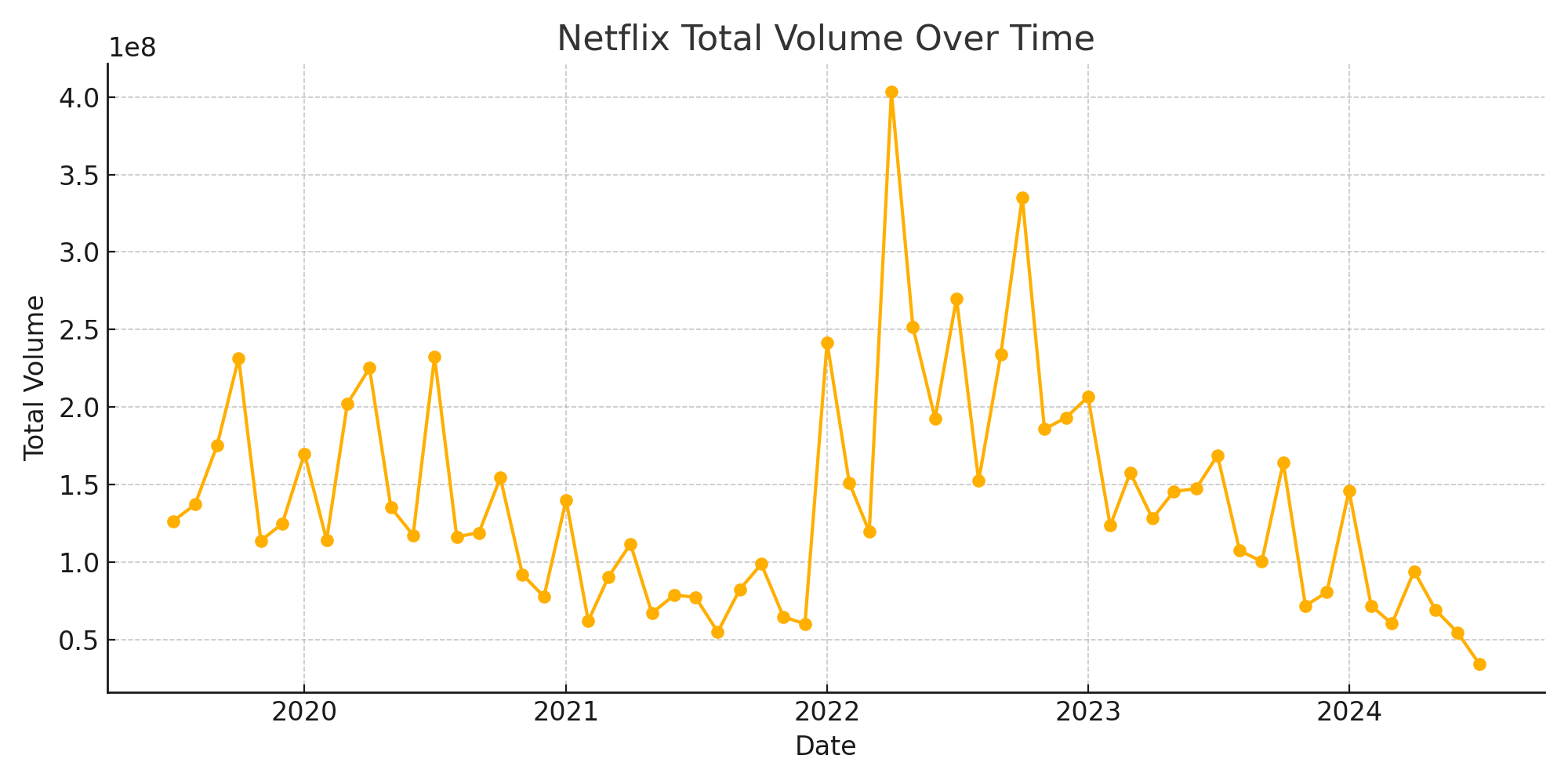
Query 4 : How has the trading volume for Netflix (NFLX) changed on a monthly basis from 2019 to current month?
Response:
```sql
SELECT
    DATE_TRUNC('month', date) AS month,
    SUM(volume) AS total_volume
FROM
    stock_data
WHERE
    ticker = 'NFLX'
    AND date BETWEEN '2019-01-01' AND '2024-07-18'
GROUP BY
    month
ORDER BY
    month;
```
After running the query, we get the output as shown below:

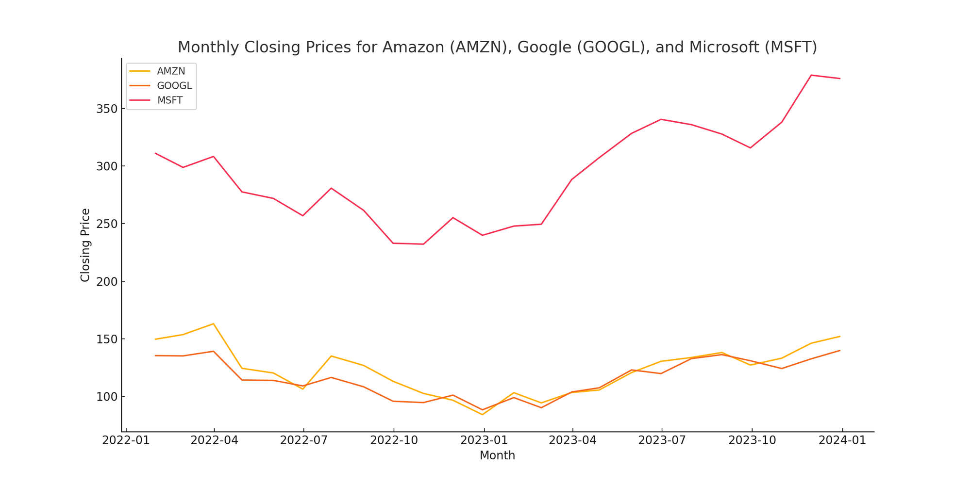
Query 5 : Please provide me the closing prices of Microsoft, Google and Amazon on last day of each month from January 2022 to December 2023
Response:
```sql
WITH last_day_per_month AS (
    SELECT
        ticker,
        DATE_TRUNC('month', date) AS month,
        MAX(date) AS last_date
    FROM
        stock_data
    WHERE
        ticker IN ('MSFT', 'GOOGL', 'AMZN')
        AND date BETWEEN '2022-01-01' AND '2023-12-31'
    GROUP BY
        ticker, month
)
SELECT
    ldm.last_date AS month,
    sd.ticker,
    sd.close AS closing_price
FROM
    last_day_per_month ldm
JOIN
    stock_data sd
ON
    ldm.ticker = sd.ticker
    AND ldm.last_date = sd.date
ORDER BY
    ldm.last_date, sd.ticker;

```
After running the query, we get the output:

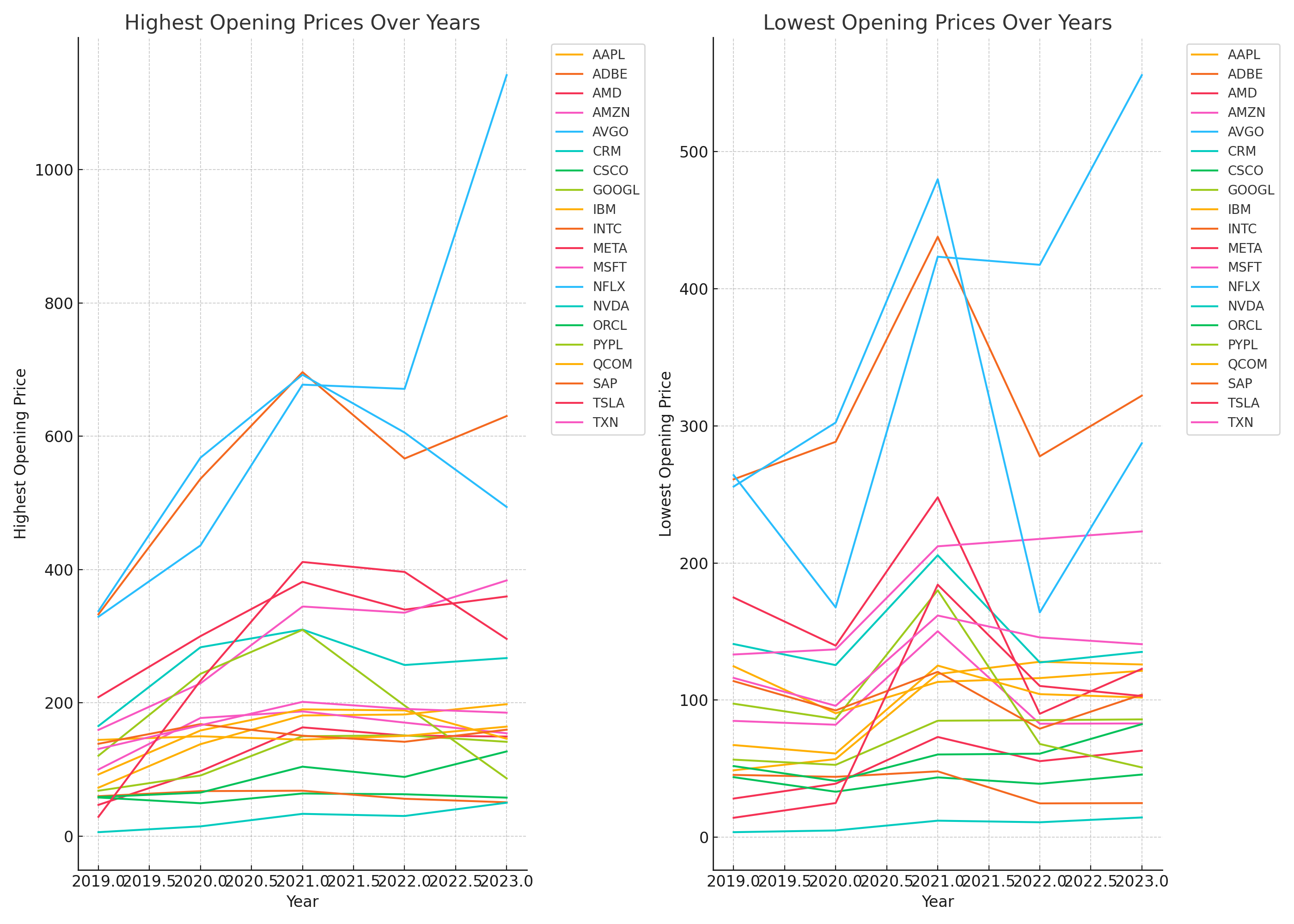
Query 6 : What were the highest and lowest opening prices for all the companies in the database for each year from 2019 to 2023?
Response:
```sql
SELECT EXTRACT(YEAR FROM date) AS year, ticker, MAX(open) AS highest_open, MIN(open) AS lowest_open
FROM stock_data
WHERE date >= '2019-01-01' AND date <= '2023-12-31'
GROUP BY year, ticker
ORDER BY year, ticker;
```
This is the result of the SQL query:

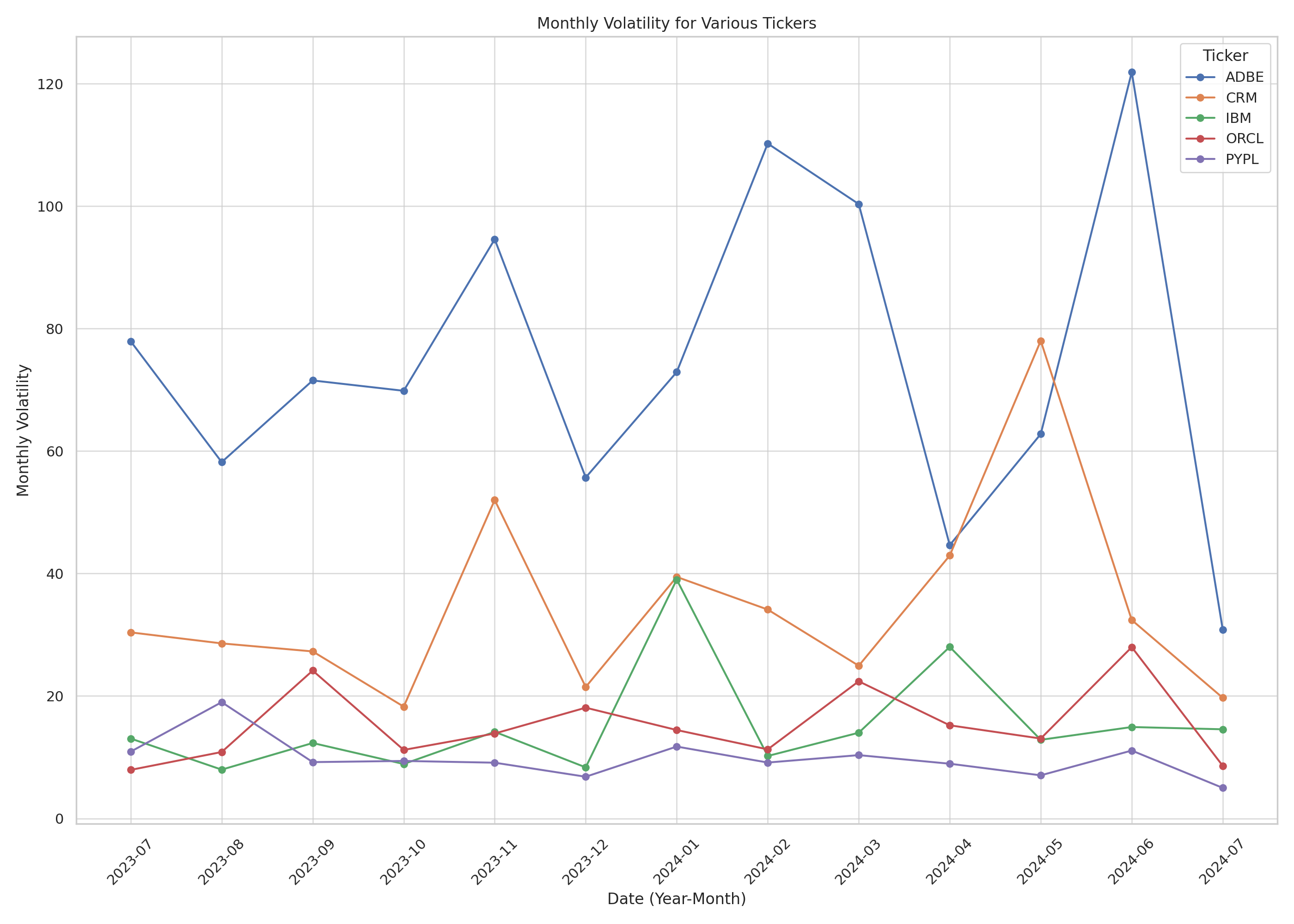
Query 7 : What is the monthly volatility, measured as the difference between the highest and lowest prices, for Oracle(ORCL), IBM(IBM), Adobe(ADBE), Paypal(PYPL) and Salesforce(CRM) from July 2023 to July 2024?
Response:
```sql
SELECT ticker,
       EXTRACT(YEAR FROM date) AS year,
       EXTRACT(MONTH FROM date) AS month,
       MAX(high) - MIN(low) AS monthly_volatility
FROM stock_data
WHERE ticker IN ('ORCL', 'IBM', 'ADBE', 'PYPL', 'CRM')
  AND date BETWEEN '2023-07-01' AND '2024-07-31'
GROUP BY ticker, year, month
ORDER BY ticker, year, month;
```
On running the query, we get the output as shown below:

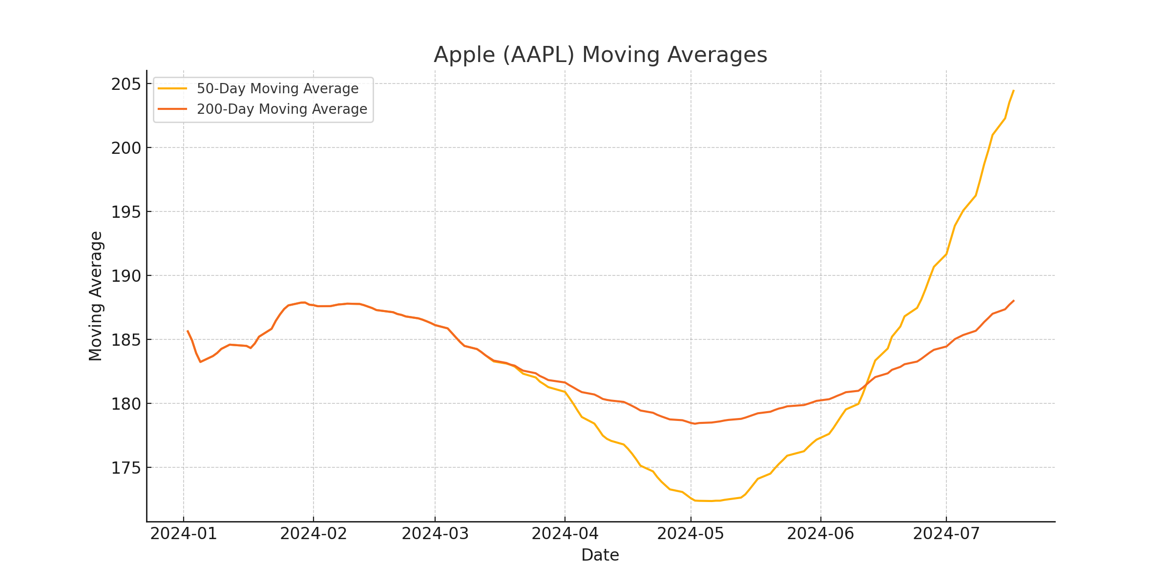
Query 8 : Calculate the 50-day and 200-day moving averages for company Apple(AAPL) from January 2024 to July 2024
Response:
```sql
WITH CalculatedAverages AS (
    SELECT
        ticker,
        date,
        AVG(close) OVER (PARTITION BY ticker ORDER BY date ROWS BETWEEN 49 PRECEDING AND CURRENT ROW) AS moving_average_50,
        AVG(close) OVER (PARTITION BY ticker ORDER BY date ROWs BETWEEN 199 PRECEDING AND CURRENT ROW) AS moving_average_200
    FROM
        stock_data
    WHERE
        ticker LIKE 'AAPL' AND
        date BETWEEN '2024-01-01' AND '2024-07-31'
)
SELECT
    ticker,
    date,
    moving_average_50,
    moving_average_200
    FROM
    CalculatedAverages
ORDER BY
    ticker,
    date;
```
After running the query, we get the output:

Using OpenAI's Assistant API to generate time series analysis
Time series analysis helps us understand data collected over time and make forecasts. With OpenAI's Assistant API, we can simplify this process by using natural language to generate and interpret analysis. The API helps you easily ask questions about data, uncover patterns and get insights making time series analysis more intuitive and efficient.
The code is shown below:
First, we'll install openai using pip
pip install openai
from openai import OpenAI

OPENAI_API_KEY = 'ENTER_YOUR_API_KEY'
client = OpenAI(api_key=OPENAI_API_KEY)
We then import the OpenAI class from the openai library and set the API key required for authentication to create an instance of the OpenAI client using this API key, enabling interaction with OpenAI's API for making requests.
#To upload a file
file = client.files.create(
    file=open("/file_name.csv", "rb"),
    purpose='assistants'
)

#Call this to get the list of all uploaded files
file_list = client.files.list()
file_id = file_list.data[0].id
This code snippet uploads a file named file_name.csv with the purpose 'assistants' using client.files.create. It then retrieves a list of all uploaded files with client.files.list() and extracts the ID of the first file in the list.
# Create the assistant
assistant = client.beta.assistants.create(
  instructions="You are an expert data analysis assistant and are extremely skilled in analyzing financial data, particularly from tabular data. Please generate basic time series statistics using Pandas and plot the time series data.",
  model="gpt-4o",
  tools=[{"type": "code_interpreter"}],
  tool_resources={
    "code_interpreter": {
      "file_ids": [file.id]
    }
  }
)
We move on to now create an assistant using the OpenAI client. It sets up the assistant with instructions to analyze financial data from tabular formats, using Pandas to generate time series statistics and plot data.
The assistant is configured with the gpt-4o model and includes a code interpreter tool, which is linked to the uploaded file for data analysis.
thread = client.beta.threads.create()
message = client.beta.threads.messages.create(
    thread_id = thread.id,
    role = 'user',
    content='Generate me basic time series statistics using Pandas and plot the time series data.  Provide a link to download the image. Provide me a link to download the script as well.'
)

run = client.beta.threads.runs.create(
    thread_id = thread.id,
    assistant_id = assistant.id,

)

run = client.beta.threads.runs.retrieve(
    thread_id = thread.id,
    run_id = run.id
)

while run.status not in ["completed", "failed"]:
  run = client.beta.threads.runs.retrieve(
    thread_id = thread.id,
    run_id = run.id
  )

  print(run.status)
  time.sleep(10)

  messages = client.beta.threads.messages.list(
    thread_id = thread.id,

)
client.beta.threads.create():Creates a new conversation thread within the OpenAI system, allowing you to send and receive messages related to a specific task.client.beta.threads.runs.create(thread_id=thread.id, assistant_id=assistant.id):Initiates a run of the assistant in the specified thread, using the given assistant ID (assistant.id).This action starts the process of executing the assistant's tasks based on the provided instructions.client.beta.threads.runs.retrieve(thread_id=thread.id, run_id=run.id):Retrieves the status of the run (run.id) in the specified thread (thread.id).This function is used to check if the run has completed or failed.time.sleep(10):Pauses execution for 10 seconds between status checks to avoid excessive polling.client.beta.threads.messages.list(thread_id=thread.id):Lists all messages within the specified thread (thread.id), allowing retrieval of responses and results once the run is complete.
Finally,
for message in messages:
    print("-" * 50)
    # Print the role of the sender
    print(f"Role: {message.role}")

    # Process each content item in the message
    for content in message.content:
        # Check if the content is text
        if content.type == 'text':
            print(content.text.value)

            # Check and print details about annotations if they exist
            if content.text.annotations:
                for annotation in content.text.annotations:
                    print(f"Annotation Text: {annotation.text}")
                    print(f"File_Id: {annotation.file_path.file_id}")
                    annotation_data = client.files.content(annotation.file_path.file_id)
                    annotation_data_bytes = annotation_data.read()


                    filename = annotation.text.split('/')[-1]

                    with open(f"{filename}", "wb") as file:
                        file.write(annotation_data_bytes)

        # Check if the content is an image file and print its file ID and name
        elif content.type == 'image_file':
            print(f"Image File ID: {content.image_file.file_id}")


    # Print a horizontal line for separation between messages
    print("-" * 50)
    print('\n')
The code processes messages by first retrieving the sender’s role with print(f"Role: {message.role}"). It then iterates through each content item in the message using for content in message.content:.
For text content, it checks with if content.type == 'text':. If true, it prints the text value using print(content.text.value). If there are annotations, the code retrieves each annotation's text and file ID. It fetches the associated file content using client.files.content(annotation.file_path.file_id), reads it into bytes, and saves the file locally with with open(f"{filename}", "wb") as file: and file.write(annotation_data_bytes).
For image content, it checks if content.type == 'image_file': and, if true, prints the image file ID with print(f"Image File ID: {content.image_file.file_id}").
After this, the image and the script would be downloaded into your folder.
These are the results:
Refer to the earlier queries that were in the previous section
- Query 4: Trading volume for Netflix (NFLX) on a monthly basis from 2019 to current month.
Generated analysis:
Generated code:
import pandas as pd
import matplotlib.pyplot as plt

# Load the CSV file
file_path = 'PATH/TO/YOUR/CSV'
df = pd.read_csv(file_path)

# Convert 'month' column to datetime
df['month'] = pd.to_datetime(df['month'], errors='coerce')

# Setting the 'month' column as the index for time series analysis
df.set_index('month', inplace=True)

# Generate basic time series statistics
time_series_stats = df.describe()
print(time_series_stats)

# Plot the time series data
plt.figure(figsize=(10, 5))
plt.plot(df.index, df['total_volume'], marker='o')
plt.title('Netflix Total Volume Over Time')
plt.xlabel('Date')
plt.ylabel('Total Volume')
plt.grid(True)
plt.tight_layout()

# Save the plot
plot_path = 'PATH/TO/SAVE/PLOT/netflix_total_volume_timeseries.png'
plt.savefig(plot_path)
plt.show()
- Similarly, for query 5: The closing prices of Microsoft, Google and Amazon on last day of each month from January 2022 to December 2023
Analysis:
Generated code:
import pandas as pd
import matplotlib.pyplot as plt

# Load the CSV file
file_path = 'file-lPcZitlATWP9bQfMIwS3ce25.csv'
data = pd.read_csv(file_path)

# Convert 'month' to datetime and set as index
data['month'] = pd.to_datetime(data['month'], format='%d-%m-%Y')
data.set_index('month', inplace=True)

# Generate basic statistics
stats = data.groupby('ticker')['closing_price'].describe()
print(stats)

# Plot time series data
fig, ax = plt.subplots(figsize=(14, 7))

for key, grp in data.groupby('ticker'):
    ax.plot(grp.index, grp['closing_price'], label=key)

ax.set_title('Monthly Closing Prices for Amazon (AMZN), Google (GOOGL), and Microsoft (MSFT)')
ax.set_xlabel('Month')
ax.set_ylabel('Closing Price')
ax.legend()
plt.grid()

# Save the plot
plot_path = 'stock_closing_prices.png'
plt.savefig(plot_path)
plt.show()
- For query 6: The highest and lowest opening prices for all the companies in the database for each year from 2019 to 2023
The analysis:
The code generated in response:
import pandas as pd
import matplotlib.pyplot as plt

# Load the CSV file
file_path = 'path/to/your/file.csv'
df = pd.read_csv(file_path)

# Generating basic statistics
stats = df.groupby('ticker').agg({'highest_open': ['min', 'max', 'mean'], 'lowest_open': ['min', 'max', 'mean']})

# Reshaping data for plotting
pivot_highest = df.pivot(index='year', columns='ticker', values='highest_open')
pivot_lowest = df.pivot(index='year', columns='ticker', values='lowest_open')

# Plotting
plt.figure(figsize=(14, 10))

# Plot highest opening prices
plt.subplot(1, 2, 1)
for column in pivot_highest:
    plt.plot(pivot_highest.index, pivot_highest[column], label=column)
plt.title('Highest Opening Prices Over Years')
plt.xlabel('Year')
plt.ylabel('Highest Opening Price')
plt.legend(bbox_to_anchor=(1.04,1), loc="upper left")

# Plot lowest opening prices
plt.subplot(1, 2, 2)
for column in pivot_lowest:
    plt.plot(pivot_lowest.index, pivot_lowest[column], label=column)
plt.title('Lowest Opening Prices Over Years')
plt.xlabel('Year')
plt.ylabel('Lowest Opening Price')
plt.legend(bbox_to_anchor=(1.04,1), loc="upper left")

# Save the plot
plt.tight_layout()
plt.savefig('timeseries_plot.png')
plt.show()

# Display the basic statistics
print(stats)
For query 7: The monthly volatility for Oracle(ORCL), IBM(IBM), Adobe(ADBE), Paypal(PYPL) and Salesforce(CRM) from July 2023 to July 2024
The graph generated:
The code generated by interpreter:
import pandas as pd
import matplotlib.pyplot as plt
import seaborn as sns

# Load the data from the CSV file
file_path = 'your_file_path.csv'  # Change this to your file path
data = pd.read_csv(file_path)

# Display basic information about the data
data_info = data.info()
data_description = data.describe()

print(data_info)
print(data_description)

# Create a plot for the time series data
plt.figure(figsize=(14, 10))
sns.set(style="whitegrid")

# Plot each ticker's volatility over time
for ticker in data['ticker'].unique():
    ticker_data = data[data['ticker'] == ticker]
    plt.plot(ticker_data['year'].astype(str) + '-' + ticker_data['month'].astype(str).str.zfill(2),
             ticker_data['monthly_volatility'], marker='o', label=ticker)

plt.title('Monthly Volatility for Various Tickers')
plt.xlabel('Date (Year-Month)')
plt.ylabel('Monthly Volatility')
plt.xticks(rotation=45)
plt.legend(title='Ticker')
plt.tight_layout()

# Save the plot as an image
plot_path = 'monthly_volatility_plot.png'
plt.savefig(plot_path)

print(f'Plot saved at {plot_path}')
Lastly for query 8: The 50-day and 200-day moving averages for company Apple(AAPL) from January 2024 to July 2024
Analysis:
Generated code:
import pandas as pd
import matplotlib.pyplot as plt

# Load the CSV file
file_path = 'file-My1EOifqGvOKd4V2jLySKqI2'
data = pd.read_csv(file_path)

# Convert the 'date' column to datetime
data['date'] = pd.to_datetime(data['date'], format='%d-%m-%Y')

# Set the 'date' column as the index
data.set_index('date', inplace=True)

# Calculate basic statistics
stats = data[['moving_average_50', 'moving_average_200']].describe()
print(stats)

# Plot the time series data
plt.figure(figsize=(12, 6))
plt.plot(data.index, data['moving_average_50'], label='50-Day Moving Average')
plt.plot(data.index, data['moving_average_200'], label='200-Day Moving Average')
plt.xlabel('Date')
plt.ylabel('Moving Average')
plt.title('Apple (AAPL) Moving Averages')
plt.legend()
plt.grid(True)

# Save the plot as an image file
plot_file_path = 'apple_moving_averages.png'
plt.savefig(plot_file_path)
plt.show()
Conclusion
Integrating AI into financial analysis represents a significant leap forward in how we approach and understand data. By combining advanced data fetching techniques with intelligent automation and sophisticated analytical tools, we can transform raw financial data into clear, actionable insights.
This synergy of technology not only simplifies complex processes but also enhances our ability to make data-driven decisions with greater precision.
As AI continues to evolve, its role in financial analysis will only grow, offering deeper insights and driving more strategic outcomes in the world of finance.
If you are looking for an AI co-pilot to learn more about public companies, then check out https://dafinchi.ai/

