BERTopic: A Comprehensive Guide to Modular Topic Modeling

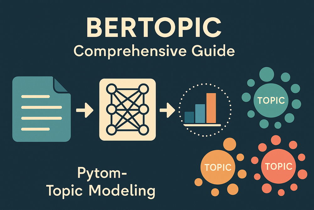
Navigating the vast sea of text data can feel overwhelming. How do you find the hidden themes in thousands of customer reviews, news articles, or research papers? Enter BERTopic, a powerful and flexible Python library designed to do just that. By leveraging cutting-edge transformer models, BERTopic moves beyond traditional topic modeling to provide more intuitive, context-aware topics.

But its real power lies in its modularity. Whether you're a data scientist looking to fine-tune every step of the process or a researcher needing to incorporate prior knowledge into your model, BERTopic offers a customizable framework to fit your needs.

If you're ready to unlock deeper insights from your text data, you've come to the right place. Dive into our comprehensive guide below, which covers everything from installation and core concepts to advanced techniques and visualization, all based on the library's own documentation.

How This Article Was Generated

This article was generated by an AI assistant. The process was initiated when we uploaded the source documentation from the BERTopic GitHub repository.

Here’s a breakdown of how the AI created this guide:

1. File Processing: The AI first processed the provided text file (maartengr-bertopic.txt) to access the complete documentation. This file was created using gitingest by compacting into a single file the source code from BERTopic Github repository.
2. Information Extraction & Structuring: It then analyzed the content, systematically extracting information corresponding to a detailed set of user-defined sections (like "Introduction," "Installation," "Core Concepts," "API and Usage," etc.).
3. Content Synthesis: Finally, the AI synthesized the extracted information into a structured, long-form article. It organized the content with headings, subheadings, code examples, and highlighted warnings, adhering strictly to the material found in the source documentation without inventing any new information.

The result is a comprehensive guide that serves as a detailed walkthrough of the BERTopic library, created by an AI to be an educational resource for developers and data scientists.

1. Introduction and Purpose

BERTopic is a Python library designed for topic modeling. It leverages transformer models (like BERT) and a class-based TF-IDF (c-TF-IDF) approach to create dense clusters allowing for easily interpretable topics while keeping important words in the topic descriptions. Its core strength lies in its

modularity, allowing users to customize nearly every step of the topic modeling pipeline.

What it does:

• Transforms documents into numerical embeddings.
• Optionally reduces the dimensionality of these embeddings.
• Clusters the embeddings to group similar documents.
• Uses a modified TF-IDF approach (c-TF-IDF) to identify important words within each cluster, thereby representing the topics.
• Offers various techniques for fine-tuning and representing these topics.

Typical Use Cases:

BERTopic is versatile due to its modular nature. Common use cases include:

• Discovering hidden themes and topics in large collections of text documents.
• Analyzing customer feedback, reviews, or survey responses.
• Understanding themes in scientific literature, news articles, or social media posts.
• Modeling topics in multimodal data (text + images).
• Guiding topic discovery using predefined seed words or existing labels (Guided, Semi-Supervised, Supervised, Manual Topic Modeling).
• Tracking how topics evolve over time (Dynamic Topic Modeling).
• Analyzing topic distributions within specific document categories (Topics per Class).

2. Installation and Setup

While the provided documentation focuses on usage and concepts, standard Python package installation methods apply. You would typically install BERTopic using pip:

pip install bertopic

Depending on the specific functionalities you intend to use (like certain embedding models, visualization tools, or GPU acceleration), you might need to install additional dependencies. Examples mentioned in the documentation include:

• SentenceTransformers: Often used for embeddings. Install via pip install sentence-transformers (or it may be installed as a core dependency).
• UMAP: Default for dimensionality reduction. Install via pip install umap-learn.
• HDBSCAN: Default for clustering. Install via pip install hdbscan.
• Scikit-learn: Required for CountVectorizer and alternative dimensionality reduction/clustering/classification models. Install via pip install scikit-learn.
• Visualization Dependencies: Plotly is used heavily. Install viapip install plotly. Jinja2 might be needed for styled dataframes. Install viapip install Jinja2. DataMapPlot is an alternative visualization. Install viapip install datamapplot.
• Specific Embedding Backends:
  • Hugging Face Transformers: pip install transformers
  • Flair: pip install flair
  • Spacy: pip install spacy and download models (e.g., python -m spacy download en_core_web_md)
  • Gensim: pip install gensim
  • TensorFlow Hub (for USE): pip install tensorflow tensorflow_hub
  • OpenAI: pip install openai
  • Cohere: pip install cohere
  • LangChain: pip install langchain
  • LiteLLM: pip install litellm
  • Llama.cpp: pip install llama-cpp-python (with hardware-specific options available)
  • ctransformers (for GGUF models like Zephyr): pip install ctransformers[cuda]
  • tiktoken (for OpenAI token counting): pip install tiktoken
  • bitsandbytes (for model quantization): pip install bitsandbytes
  • FastEmbed: pip install fastembed
  • Model2Vec: pip install model2vec or pip install model2vec[distill]
• GPU Acceleration (cuML): Requires a specific setup detailed in the documentation involving cudf, cuml, cugraph, and cupy.

3. Core Concepts

BERTopic's architecture is designed to be modular, allowing components to be swapped or customized. The main steps are:

1. Document Embedding:
   • Purpose: Convert text documents (or images) into high-dimensional numerical vectors (embeddings) that capture semantic meaning.
   • Default: Uses sentence-transformers (specifically "all-MiniLM-L6-v2").
   • Modularity: BERTopic supports a wide range of embedding models, including Hugging Face Transformers, Flair, Spacy, USE, Gensim Word Embeddings, TF-IDF, and even external APIs like OpenAI and Cohere. You can also provide pre-calculated embeddings. For multimodal data, specific backends likeMultiModalBackend handle text and images.
2. Dimensionality Reduction:
   • Purpose: Reduce the high dimensionality of embeddings to combat the "curse of dimensionality" and make clustering more effective.
   • Default: Uses UMAP (Uniform Manifold Approximation and Projection) because it's good at capturing both local and global structure in lower dimensions.
   • Modularity: Any scikit-learn compatible dimensionality reduction technique (with .fit() and .transform() methods) can be used, such as PCA or TruncatedSVD. GPU-accelerated UMAP via cuML is also supported. This step can also be skipped entirely.
3. Clustering:
   • Purpose: Group the reduced embeddings into clusters, where each cluster represents a potential topic.
   • Default: Uses HDBSCAN (Hierarchical Density-Based Spatial Clustering of Applications with Noise) because it can find clusters of varying densities and doesn't require specifying the number of clusters beforehand. It also identifies outliers (documents not assigned to any topic).
   • Modularity: Any clustering algorithm with .fit() and .predict() methods (and a .labels_ attribute) can be substituted, such as k-Means or Agglomerative Clustering. GPU-accelerated HDBSCAN via cuML is supported.
4. Topic Representation (c-TF-IDF):
   • Purpose: Generate meaningful representations (keywords) for each cluster (topic).
   • Method: BERTopic employs a class-based TF-IDF (c-TF-IDF) mechanism. Instead of calculating TF-IDF scores for words across individual documents, it treats all documents within a cluster as a single "document". It then calculates the frequency of words within that "topic document" (term frequency, tf) and compares it against the frequency across all topics (inverse document frequency, idf). This highlights words that are important to a specific topiccompared to other topics.
   • Formula:
     • Term Frequency (tf): Frequency of word x in class c, L1-normalized to account for topic size differences.
     • Inverse Document Frequency (idf): log(1 + A / f_x), where A is the average number of words per class and f_x is the frequency of word x across all classes.
     • c-TF-IDF Score: tf * idf.
   • Underlying Tool: The CountVectorizer from scikit-learn is used to tokenize documents and create the initial bag-of-words matrix needed for c-TF-IDF.
   • Modularity: The ClassTfidfTransformer can be customized with parameters like bm25_weighting (uses BM25 instead of standard IDF) and reduce_frequent_words (applies square root weighting to term frequencies). TheCountVectorizer itself can also be heavily customized (e.g., ngram_range, stop_words, min_df) or replaced.
5. Topic Representation Fine-tuning (Optional):
   • Purpose: Further refine or diversify the keywords generated by c-TF-IDF using various techniques.
   • Methods: BERTopic offers several representation_model options, including KeyBERTInspired (semantic similarity), PartOfSpeech (POS tagging), Maximal Marginal Relevance (MMR for diversity), ZeroShotClassification (assigning predefined labels), and interfaces to Large Language Models (LLMs) like OpenAI's GPT, Cohere, Llama 2, Zephyr, or models via LangChain/LiteLLM for generating labels or summaries. These can even be chained.

Diagrammatic Representation:

The documentation frequently uses SVG diagrams to illustrate the modular pipeline. While I cannot display SVGs, the core idea is a sequence:

Documents -> Embeddings -> [Dim Reduction] -> Clustering -> [Topic Representation]

Where [Dim Reduction] and Clustering can be swapped or modified, and [Topic Representation] involves c-TF-IDF potentially followed by fine-tuning models.

4. API and Usage

The central class in the library is bertopic.BERTopic.

Initialization (BERTopic(...))

The constructor accepts various parameters to customize the pipeline components:

• embedding_model: An embedding model instance (e.g., from sentence-transformers, flair, spacy) or a string pointing to a SentenceTransformer model. Can also be custom backends likeOpenAIBackend, CohereBackend, MultiModalBackend etc., or even scikit-learn pipelines.
• umap_model: A dimensionality reduction model instance (needs .fit() and .transform()), like UMAP() or PCA(). Usebertopic.dimensionality.BaseDimensionalityReduction() to skip this step.
• hdbscan_model: A clustering model instance (needs .fit(), .predict(), .labels_), like HDBSCAN() or KMeans(). Usebertopic.cluster.BaseCluster() to skip clustering if providing manual labels. For supervised classification, pass a classifier (e.g.,LogisticRegression()) here.
• vectorizer_model: An instance of sklearn.feature_extraction.text.CountVectorizer or compatible classes like bertopic.vectorizers.OnlineCountVectorizer.
• ctfidf_model: An instance of bertopic.vectorizers.ClassTfidfTransformer. Can be customized withbm25_weighting or reduce_frequent_words.
• representation_model: A single representation model instance (e.g., KeyBERTInspired(), PartOfSpeech(), OpenAI()) or a list for chaining, or a dictionary for multi-aspect modeling.
• top_n_words: Number of words per topic representation (default is 10).
• min_topic_size: Minimum size of a cluster to be considered a topic (passed to HDBSCAN, default influences clustering).
• nr_topics: Reduce the number of topics after clustering by merging the most similar ones until nr_topics remain. Advised to control topic number viamin_topic_size instead.
• calculate_probabilities: Whether HDBSCAN should calculate document-topic probabilities (can be slow).
• seed_topic_list: A list of lists containing seed keywords for Guided Topic Modeling.
• zeroshot_topic_list: List of predefined topic labels for Zero-Shot Topic Modeling.
• zeroshot_min_similarity: Minimum similarity score for assigning a document to a zero-shot topic.
• verbose: Whether to print progress messages.

Fitting (.fit(docs, y=None, embeddings=None, images=None))

• Trains the model on the provided documents (docs).
• docs: A list of document strings.
• y (optional): A list of pre-defined labels/classes for each document. Used for supervised, semi-supervised, or manual topic modeling.
• embeddings (optional): Pre-calculated document embeddings. If provided, the embedding_model step is skipped during fitting.
• images (optional): A list of images (PIL images or paths) corresponding to docs for multimodal modeling. If only images are provided,docs should be None.
• Returns: self (the fitted model object).

Transforming (.fit_transform(docs, y=None, embeddings=None, images=None) / .transform(docs, embeddings=None, images=None))

• .fit_transform: Fits the model and then assigns topics to the input documents. Returns topics, probabilities.
• .transform: Assigns topics to new, unseen documents based on the already fitted model. Requires pre-calculated embeddings if the model was saved using safetensors/pytorch or if a custom embedder without .embed() is used. Returns topics, probabilities.
• Returns:
  • topics: A list of topic assignments for each document. Outliers are typically assigned topic -1.
  • probabilities (or probs): If calculate_probabilities=True during init (and HDBSCAN is used), this is a matrix of probabilities for each document belonging to each topic. Otherwise, it might beNone or estimated differently depending on the setup. For models saved with safetensors/pytorch, transform probabilities are based on cosine similarity to topic embeddings.

Getting Topic Information

• .get_topic_info(): Returns a pandas DataFrame with information about each topic, including Topic ID, Count (number of documents), Name (default: ID_word1_word2_word3), Representation (list of top words), Representative_Docs, and potentially CustomName if labels were set, or columns for multi-aspect representations.
• .get_topic(topic_id): Returns the list of (word, score) tuples for a specific topic ID. Iffull=True is used with multi-aspect models, returns a dictionary with representations for each aspect.
• .get_topics(): Returns a dictionary mapping topic IDs to their list of (word, score) tuples.
• .get_document_info(docs): Returns a DataFrame mapping input documents to their assigned Topic, Name, Top_n_words, Probability, Representative_document status.
• .topic_aspects_: A dictionary holding the representations for different aspects if multi-aspect modeling was used.

Updating and Modifying Topics

• .update_topics(docs, topics=None, vectorizer_model=None, ctfidf_model=None, representation_model=None): Updates topic representations after fitting, without re-clustering. Useful for tuning representations with different vectorizer_model settings or applying new representation models. Can also update topics based on modified assignments (e.g., after outlier reduction).
• .reduce_outliers(docs, topics, strategy="probabilities"|"embeddings"|"distributions", ...) : Assigns outlier documents (topic -1) to actual topics based on specified strategy. Requires recalculating topic representations using.update_topics afterwards if assignments change.Warning: Can cause issues with later topic reduction/merging.
• .reduce_topics(docs, topics, nr_topics=None): Reduces the number of topics by merging the least frequent topics with their most similar counterparts until nr_topics remain or based on a similarity threshold.
• .merge_topics(docs, topics_to_merge): Manually merges specified topics. Input topics_to_merge is a list of topic IDs (e.g., [1, 2]) or a list of lists for multiple merges (e.g., [[1, 2], [3, 4]]). Updates the model's representations.
• .set_topic_labels(topic_labels): Manually sets custom labels for topics. Input topic_labels is a dictionary mapping topic ID to label string (e.g., {1: "Space Travel", 7: "Religion"}). Can also use labels generated from other representation aspects. Updates theCustomName column in .get_topic_info().

Other Key Methods

• .find_topics(search_term, top_n=5): Finds topics most similar to a given search term based on embedding similarity. Requires anembedding_model. Returnssimilar_topics (list of topic IDs) and similarity (list of scores).
• .topics_over_time(docs, timestamps, ...): Performs Dynamic Topic Modeling (DTM) to track topic frequencies over time. Requires timestamps for each document. Returns a DataFrame.
• .topics_per_class(docs, classes): Calculates topic representations specific to different classes/categories within the data. Returns a DataFrame.
• .hierarchical_topics(docs, linkage_function=None): Computes a potential hierarchy of topics based on c-TF-IDF similarity. Returns a DataFrame describing merged topics at different levels.
• .get_topic_tree(hierarchical_topics): Generates a text-based tree representation of the topic hierarchy.
• .approximate_distribution(docs, ...): Estimates the topic distribution within each document using a sliding window approach over tokenized text. Can also calculate token-level distributions. Faster alternative tocalculate_probabilities=True.
• .partial_fit(docs): Incrementally updates the model with new batches of documents (Online Topic Modeling). Requires specific sub-models that support incremental learning (e.g.,IncrementalPCA, MiniBatchKMeans, OnlineCountVectorizer).Note: Cannot be used after .fit().
• .merge_models(topic_models, min_similarity=0.7): Merges multiple fitted BERTopic models sequentially into a single model. Compares topic embeddings; dissimilar topics from later models are added to the first model.min_similarity controls the threshold.
• .save(...) & .load(...): Saves and loads models. Supports safetensors, pytorch, and pickle serialization.safetensors is generally recommended. Can push to/load from HuggingFace Hub using.push_to_hf_hub(...).

Visualization Methods

BERTopic includes several built-in visualization methods using Plotly (interactive) or DataMapPlot (static/interactive):

• .visualize_topics(): 2D interactive plot of topics based on c-TF-IDF embeddings.
• .visualize_documents(docs, embeddings=None, reduced_embeddings=None, custom_labels=None, hide_document_hover=False): 2D interactive plot of documents, colored by topic. Hovering shows document content or custom labels (e.g., titles). Can use originalembeddings or pre-computed reduced_embeddings.
• .visualize_document_datamap(docs, embeddings=None, reduced_embeddings=None, interactive=False): Static or interactive DataMapPlot visualization of documents.
• .visualize_hierarchy(hierarchical_topics=None): Interactive dendrogram showing the computed topic hierarchy. Requires running.hierarchical_topics() first unless passed directly.
• .visualize_hierarchical_documents(docs, hierarchical_topics, embeddings=None, reduced_embeddings=None): 2D plot showing documents colored by their position in the topic hierarchy at different levels.
• .visualize_barchart(): Bar chart showing c-TF-IDF scores for top terms within selected topics.
• .visualize_heatmap(): Heatmap showing cosine similarity between topic embeddings. Can cluster topics for better structure.
• .visualize_term_rank(log_scale=False): Plots c-TF-IDF scores vs. term rank to help identify optimal number of words per topic (elbow method).
• .visualize_topics_over_time(topics_over_time, topics=None): Interactive line plot showing topic frequency evolution over time. Requires running.topics_over_time() first.
• .visualize_topics_per_class(topics_per_class, top_n_topics=None): Bar chart comparing topic representations across different classes. Requires running.topics_per_class() first.
• .visualize_distribution(probabilities_or_distribution): Visualizes the probability or topic distribution for a single document.
• .visualize_approximate_distribution(doc, topic_token_distribution): Shows topic distributions at the token level for a single document. Requires running.approximate_distribution() with calculate_tokens=True.

5. Advanced Techniques

BERTopic's modularity allows for numerous advanced configurations and extensions:

• Custom Components: Replace default embedding, dimensionality reduction, clustering, or vectorizer models with custom implementations or alternatives from libraries like scikit-learn, Flair, Spacy, etc., as long as they adhere to the expected API (e.g., .fit(), .transform()). Create custom backends usingbertopic.backend.BaseEmbedder. Create custom representation models usingbertopic.representation._base.BaseRepresentation.
• Multi-Aspect Topic Modeling: Generate multiple representations (e.g., keywords, POS-filtered phrases, summaries via LLM) for each topic simultaneously by passing a dictionary of representation models to representation_model during initialization.
• Multimodal Topic Modeling: Model topics using both text and images, or images only. Requires using aMultiModalBackend for embedding and VisualRepresentation models.
• Guided/Seeded Topic Modeling: Nudge the model towards predefined topics by providing seed keywords via the seed_topic_list parameter. This influences both the semi-supervised dimensionality reduction and the c-TF-IDF calculation.
• Seed Word Weighting: Increase the importance of specific domain words in the c-TF-IDF calculation (and thus topic representations) using the seed_words and seed_multiplier parameters in ClassTfidfTransformer.
• Semi-Supervised Topic Modeling: Guide topic formation using known labels for a subset (or all) of the documents by passing labels to the y parameter in .fit() or .fit_transform(). Unlabeled documents are typically marked with -1.
• Supervised Topic Modeling / Classification: Replace the clustering step with a classifier (e.g., LogisticRegression) passed to hdbscan_model and provide labels via y. The model learns to classify documents into the provided categories, and c-TF-IDF generates topic representations for these categories. Dimensionality reduction is typically skipped.
• Manual Topic Modeling: If clusters/labels are already known, skip embedding, dimensionality reduction, and clustering by passing empty base models and providing the labels via y. BERTopic then only performs c-TF-IDF to generate topic representations for the predefined groups.
• Online/Incremental Topic Modeling: Update the model with new data batches using .partial_fit(). Requires sub-models supporting incremental learning (e.g.,IncrementalPCA, MiniBatchKMeans, OnlineCountVectorizer). Can use frameworks like River for dynamic cluster creation.Warning: Different from .fit(); track topics manually if needed for later analysis.
• Merging Models: Combine multiple pre-trained BERTopic models using BERTopic.merge_models(). Useful for handling incoming data without full online learning or combining models with different settings. Can help discover new topics appearing in later data batches.
• Outlier Reduction: Assign outlier documents (topic -1) to existing topics using .reduce_outliers() based on different strategies (probabilities, embeddings, distributions).
• Topic Reduction/Merging: Automatically reduce the number of topics using .reduce_topics() or manually merge specific topics using .merge_topics().
• Hierarchical Topic Modeling: Explore potential relationships between topics by clustering their c-TF-IDF representations using .hierarchical_topics(). Visualize with.visualize_hierarchy() or .get_topic_tree().
• Dynamic Topic Modeling (DTM): Analyze topic evolution over time using .topics_over_time(). Requires document timestamps.
• Topics per Class: Analyze how topic representations differ across predefined document categories using .topics_per_class().
• Approximating Distributions: Estimate document-topic distributions quickly using .approximate_distribution() as an alternative to calculate_probabilities=True. Can operate at the token level.

6. Comparison or Positioning

The provided documentation focuses primarily on BERTopic's own functionalities and modularity rather than direct comparisons with other libraries (like LDA, NMF, etc.). However, some positioning can be inferred:

• Leverages Transformers: Unlike traditional methods like LDA which rely on bag-of-words from the start, BERTopic utilizes powerful pre-trained transformer embeddings (like Sentence-BERT) to capture semantic meaning before clustering. This is a key differentiator.
• Modularity as a Core Principle: BERTopic emphasizes the ability to swap components (embedding, dimensionality reduction, clustering, representation), positioning it as a flexible framework rather than a single fixed algorithm. This allows adaptation to diverse use cases and integration of new state-of-the-art techniques in any module.
• Focus on Interpretability: While leveraging complex embeddings, the final topic representation relies on the interpretable c-TF-IDF mechanism, which aims to produce coherent and easily understandable keywords. Various fine-tuning representation models (KeyBERTInspired, POS, MMR, LLMs) further enhance interpretability.
• Handles Outliers: Unlike methods like k-Means which force every document into a cluster, the default HDBSCAN allows for outliers (noise points), which can lead to more coherent topic clusters. BERTopic provides methods to explicitly handle these outliers if needed.
• Beyond Traditional Text: Extends to multimodal (text+image, image-only) topic modeling.
• Supervised & Guided Capabilities: Integrates supervised, semi-supervised, and guided approaches, allowing users to incorporate prior knowledge or existing labels, differentiating it from purely unsupervised methods.
• Alternative Online Approach: While offering .partial_fit for incremental learning, it also suggests .merge_models as a potentially more flexible alternative for handling new data, especially when using default UMAP/HDBSCAN.

7. Best Practices

The documentation highlights several best practices, particularly in best_practices.md, aimed at improving topic quality and reproducibility:

1. Pre-calculate Embeddings: Compute document embeddings once before training BERTopic, especially if iterating over parameters. Pass the embeddings via the embeddings argument in .fit() or .fit_transform() to save significant computation time.
2. Choose Embedding Models Wisely: Select high-quality embedding models. The MTEB leaderboard is a good resource for finding state-of-the-art models compatible with SentenceTransformers.all-MiniLM-L6-v2 is a good default.
3. Prevent Stochastic Behavior (Reproducibility): Set a random_state for the UMAP model (umap.UMAP(..., random_state=42)) before passing it to BERTopic to ensure reproducible results, as UMAP is stochastic by default. Also setrandom_state for HDBSCAN or other stochastic components if used.
4. Control Number of Topics via Clustering: Instead of relying solely on nr_topics (which merges topics post-creation), control the number of topics primarily through the clustering algorithm's parameters. For the default HDBSCAN, adjust min_cluster_size: higher values lead to fewer topics, lower values lead to more.min_cluster_size=150 was used as an example to avoid micro-clusters. Ensureprediction_data=True is set for HDBSCAN if using .transform or probability calculations later.
5. Improve Default Representation (CountVectorizer): Tune the CountVectorizer used for c-TF-IDF after initial training using .update_topics(). Common improvements include:
   • Removing stop words (stop_words="english").
   • Ignoring infrequent words (min_df=...).
   • Increasing the n-gram range (ngram_range=(1, 2) or (1, 3)) to include multi-word phrases, often combined with stop word removal.
6. Explore Additional Representations: Use representation_model to try different fine-tuning techniques (KeyBERTInspired, POS, MMR, LLMs) simultaneously via multi-aspect modeling for diverse perspectives on topic descriptions.
7. Use Custom Labels: Improve interpretability by assigning meaningful labels using .set_topic_labels(), either manually or based on alternative representations (like KeyBERT or LLM outputs). Usecustom_labels=True in visualization functions to display them.
8. Approximate Distributions: If calculating exact probabilities (calculate_probabilities=True) is too slow or not possible (e.g., with non-HDBSCAN clusterers), use .approximate_distribution() for a fast estimation of document-topic distributions.
9. Handle Outliers Strategically: Use .reduce_outliers() if you need all documents assigned to a topic. Be aware of potential issues if subsequent topic reduction/merging is performed.
10. Effective Visualizations:
    • Use visualize_topics() and visualize_hierarchy() for topic-level understanding.
    • Use visualize_documents() for document-level insights. Pre-calculating reduced_embeddings speeds this up. Usecustom_labels to show titles instead of full documents on hover. Be mindful that 2D is an approximation. Hide hover/annotations for large datasets if needed.
11. Prefer safetensors for Serialization: When saving models, use serialization="safetensors" for smaller, safer, and faster models, especially for sharing or production. Remember to specifysave_ctfidf=True and potentially save_embedding_model (as a string pointer).
12. Faster Inference with safetensors: Loading a model saved with safetensors skips dimensionality reduction and clustering during .transform(), using topic embedding similarity instead, which is significantly faster.
13. Sentence Splitting for Large Documents: For very long documents, consider splitting them into sentences or paragraphs before feeding them to BERTopic (e.g., using nltk.sent_tokenize).

Note: While these are termed "best practices," they might not be universally optimal for every use case. Fine-tuning based on specific needs is encouraged.

8. Visualizations or Outputs

BERTopic provides a rich suite of visualization tools, primarily using Plotly for interactivity, to help understand and validate the generated topics and document assignments.

• .visualize_topics(): Displays topics as circles in a 2D space, sized by frequency and positioned based on similarity (derived from c-TF-IDF embeddings reduced with UMAP). Hovering shows topic words and size; a slider can highlight specific topics. (Similar to LDAvis).
• .visualize_documents(): Plots individual documents in 2D space (embeddings reduced via UMAP), colored by their assigned topic. Allows exploration of cluster coherence and potential misassignments. Hovering reveals document content or custom text (like titles). Can be computationally intensive; options exist to hide hover information for large datasets.Warning: 2D projection is an approximation of high-dimensional space.
• .visualize_document_datamap(): Creates a static or interactive DataMapPlot, offering an alternative document visualization.
• .visualize_hierarchy(): Shows the potential hierarchical structure of topics as an interactive dendrogram. Hovering over nodes reveals the merged topic representation at that level. Requires running.hierarchical_topics() first.
• .visualize_hierarchical_documents(): Plots documents colored according to the hierarchical topic structure, visualizing topic splits and merges across the document space.
• .visualize_barchart(): Displays bar charts comparing the c-TF-IDF scores of the top terms for selected topics, aiding in topic comparison and interpretation.
• .visualize_heatmap(): Generates a heatmap showing the cosine similarity between topic embeddings (c-TF-IDF based or document-embedding based), revealing clusters of related topics. Ordering topics by similarity (n_clusters parameter) enhances readability.
• .visualize_term_rank(): Plots the c-TF-IDF score decline as more terms are added to a topic's representation. Useful for selecting an appropriate number of words per topic via the elbow method.log_scale=True can improve visibility.
• .visualize_topics_over_time(): Visualizes the frequency and evolution of topics over time based on Dynamic Topic Modeling results. Interactive hovering shows time-specific topic words.
• .visualize_topics_per_class(): Compares topic representations across different predefined classes using bar charts, showing how the same general topic might be expressed differently by various groups.
• .visualize_distribution(): Creates a bar chart showing the probability distribution (from HDBSCAN) or approximate topic distribution (from .approximate_distribution) for a single document.
• .visualize_approximate_distribution(): Displays topic distributions at the token level within a document as a styled DataFrame (requires Jinja2).

These visualizations are crucial for exploring the model's output, understanding topic relationships, assessing document assignments, and communicating results effectively.

9. Troubleshooting and Gotchas

The documentation provides several notes, tips, and warnings indicating potential issues or areas requiring careful consideration:

• Stochasticity: UMAP (default dimensionality reduction) is stochastic. Use random_state for reproducibility. HDBSCAN can also have stochastic elements depending on parameters.
• Computational Cost:
  • Embedding generation can be costly, especially for large datasets or complex models. Pre-calculating embeddings is recommended.
  • Calculating exact probabilities (calculate_probabilities=True) with HDBSCAN can significantly slow down training. cuML's HDBSCAN can speed this up on GPUs, but as of v0.13, calculating probabilities forunseen data with cuML HDBSCAN was not supported..approximate_distribution is a faster alternative.
  • Using embedding_model for .approximate_distribution (use_embedding_model=True) is much slower than the default c-TF-IDF comparison.
  • Visualizing documents (.visualize_documents) involves recomputing or reducing embeddings and can be expensive. Pre-reducing embeddings helps. Saving visualizations with full document hover info can create large files.
  • Using TF-IDF embeddings can be slow during the .fit_transform (dimensionality reduction) step, although embedding creation is fast. The inverse is true for transformer embeddings.
• Parameter Sensitivity:
  • min_cluster_size (HDBSCAN) strongly influences the number of topics.
  • nr_topics merges topics after creation, which might be less ideal than controlling via clustering parameters.
  • min_similarity in .merge_models affects how many topics are merged versus kept separate.
  • zeroshot_min_similarity requires experimentation based on the embedding model used.
• Model Component Compatibility:
  • Some clustering algorithms (like Agglomerative Clustering) lack a .predict() method, causing errors if .transform() is used later.
  • Scikit-learn Pipeline objects used as embedding models might not support .partial_fit() for online learning. Scikit-learn embedding backends also do not support word-level representation models.
  • cuML HDBSCAN (as of v0.13) did not support probability calculation during .transform.
• Interpretation Caveats:
  • Visualizing documents/topics in 2D is an approximation and involves significant information loss from the original high-dimensional space.
  • Topic probability distributions (probs) show model confidence, not necessarily the frequency distribution of topics within a document..approximate_distribution provides a frequency-based estimate.
• Updating/Modifying Topics: Updating topics after outlier reduction (.update_topics(docs, topics=new_topics)) can lead to errors if topic reduction or merging is performed afterwards, due to ambiguity in mapping reduced outliers.
• Online Learning (.partial_fit):
  • Cannot be used after .fit() has been called.
  • Requires sub-models that support incremental updates. Standard UMAP/HDBSCAN do not.
  • Only the most recent batch of documents is tracked internally by default. For use cases needing access to all topic assignments (like hierarchical modeling), manually collect topic_model.topics_ after each partial_fit call.
• Serialization:
  • pickle is convenient but less safe and creates large files.
  • safetensors/pytorch are preferred (smaller, safer) but do not save dimensionality reduction/clustering models. Inference (.transform) works differently for these saved models (cosine similarity).
  • Strict version control for dependencies is crucial, especially for pickle. Models saved with one BERTopic version may not load in another.
  • Embedding models might need to be loaded separately when using safetensors/pytorch if they are not standard SentenceTransformer models loadable via string pointers.
• Manual/Supervised Modeling: The resulting topics mapping might differ from the input y mapping. Use topic_model.topic_mapper_.get_mappings() to reconcile them if needed.
• Dependencies: Specific features require specific installations (e.g., Jinja2 for styled dataframes, cuML for GPU acceleration, various embedding backends).

10. Conclusion

BERTopic presents a powerful, flexible, and modern approach to topic modeling. Its modular architecture allows users to tailor the process to specific needs, incorporating state-of-the-art embedding models, dimensionality reduction techniques, and clustering algorithms.

Key Strengths:

• High-Quality Embeddings: Leverages transformer models for semantically rich document representations.
• Modularity: Offers extensive customization by allowing users to swap pipeline components.
• Interpretability: Uses c-TF-IDF for generating coherent keywords, further refinable with various representation models, including LLMs.
• Versatility: Supports unsupervised, guided, semi-supervised, supervised, online, dynamic, multimodal, and multi-aspect topic modeling.
• Visualization: Provides a comprehensive suite of interactive tools for exploration and validation.
• Efficiency Options: Offers methods like pre-calculating embeddings, .approximate_distribution, and safetensors serialization for improved speed and reduced memory usage.

Ideal Scenarios:

BERTopic excels when:

• High-quality, semantically meaningful topics are desired.
• Flexibility and customization of the topic modeling pipeline are needed.
• Access to state-of-the-art embedding models is beneficial.
• Prior knowledge (seed words, labels) needs to be incorporated.
• Analyzing topic evolution or differences across classes is required.
• Visual exploration and validation of topics and document assignments are important.
• Working with multimodal data (text and images).

By understanding its core concepts, API, and advanced features, users can effectively leverage BERTopic to uncover valuable insights from diverse datasets. Remember to consult the best practices and be mindful of potential gotchas for optimal results.