Learn about Gradient Boosting
This article gives you a tour through one of the most powerful ML algorithms of all time, 'Gradient Boosting'. Read on, to learn the workings, pros, and cons & more.

Introduction
Every person from the data field might have heard the term ' Gradient Boosting' and that Gradient Boosting is one of the most powerful and highly used algorithms in the Machine Learning world.
But what really is Gradient Boosting?
Gradient Boosting is used for regression problems and classification as well. We make an accurate predictor by combining many shallow trees or weak learners together.
Textbook definition aside, if you are thinking what does the term boosting refer to? Well, boosting is an algorithm of machine learning in which the weak learners are transformed into strong learners. We have sequential predictions in boosting and each subsequent predictor learns from the errors of the previous one. In this category, the gradient boosting method is used.
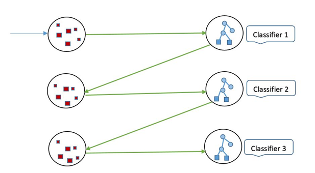
Let’s have a look at the graphical representation of Sequential Boosting.
How does Gradient Boosting work?
The following elements are included in Gradient Boosting:
- A loss function to be optimized.
- A weak learner to make predictions.
- An additive model to add weak learners to minimize the loss function.
Now we’ll discuss in detail the working of GB by defining the working of its elements.
• Loss Function
The loss function looks different for each problem depending on the problem. For regression, it uses squared error, and for classification it uses, logarithmic loss. The loss function must be differentiable.
A benefit of the gradient boosting framework is that a new boosting algorithm does not have to be derived for each loss function that may want to be used, instead, it is a generic enough framework that any differentiable loss function can be used.
• Weak Learner
Now that we’ve learned about loss function, let’s plunge into the weak learners.
We use Decision trees as the Weak learner in Gradient Boosting. Specifically, regression trees are used that output real values for splits and whose output can be added together, allowing subsequent models outputs to be added and “correct” the residuals in the predictions.
Trees are constructed in a greedy manner. Yes, that's right. Trees are constructed in a greedy manner for choosing the best split points based on purity scores like Gini or to minimize the loss.
Initially, such as in the case of AdaBoost, very short decision trees were used that only had a single split, called a decision stump. Larger trees can be used generally with 4-to-8 levels.
It is common to constrain the weak learners in specific ways, such as a maximum number of layers, nodes, splits, or leaf nodes. This is to ensure that the learners remain weak, but can still be constructed in a greedy manner.
Ok, enough about Weak Learners, now we should move to the next element.
• Additive Model
Trees are added one at a time and the existing trees in the model are not changed in an additive model. A gradient descent procedure minimizes the loss when adding trees.
Traditionally, gradient descent is used to minimize a set of parameters, such as the coefficients in a regression equation or weights in a neural network. After calculating error or loss, the weights are updated to minimize that error.
Instead of parameters, we have weak learner sub-models or more specifically decision trees. After calculating the loss, to perform the gradient descent procedure, we must add a tree to the model that reduces the loss (i.e. follow the gradient). We do this by parameterizing the tree, then modifying the parameters of the tree, and moving in the right direction by (reducing the residual loss.
Generally, this approach is called functional gradient descent or gradient descent with functions.
The output for the new tree is then added to the output of the existing sequence of trees in an effort to correct or improve the final output of the model.
A fixed number of trees are added or training stops once loss reaches an acceptable level or no longer improves on an external validation dataset.
What are Hyperparameters?
We construct many models in GB. A simple GBM model contains two categories of hyperparameters:
Boosting hyperparameters and tree-specific hyperparameters. For the improvement of model performance, values of the following can be twisted.
Boosting Hyperparameters
The two main boosting hyperparameters include the number of trees and the learning rate. Let’s discuss them in detail.
• Number of Trees
The number of trees refers to the total number of trees in the sequence or ensemble. The averaging of independently grown trees in bagging and random forests makes it very difficult to overfit with too many trees.
However, GBMs function differently as each tree is grown in sequence to fix up the past tree’s mistakes. For example, in regression, GBMs will chase residuals as long as you allow them to. Also, depending on the values of the other hyperparameters, GBMs often require many trees (it is not uncommon to have many thousands of trees) but since they can easily overfit we must find the optimal number of trees that minimize the loss function of interest with cross-validation.
• Learning Rate
The learning rate determines the contribution of each tree on the final outcome and controls how quickly the algorithm proceeds down the gradient descent (learns).
Values range from 0–1 with typical values between 0.001–0.3. Smaller values make the model robust to the specific characteristics of each individual tree, thus allowing it to generalize well. Smaller values also make it easier to stop prior to overfitting.
However, they increase the risk of not reaching the optimum with a fixed number of trees and are more computationally demanding.
This hyperparameter is also called Shrinkage. Generally, the smaller this value, the more accurate the model can be but also will require more trees in the sequence.
Tree-specific Hyperparameters
There are also two main types of tree hyperparameters.
The two main tree hyperparameters in a simple GBM model include tree depth and the minimum number of observations in terminal nodes.
• Tree Depth
Tree depth controls the depth of the individual trees. Typical values range from a depth of 3–8 but it is not uncommon to see a tree depth of 1 (J. Friedman, Hastie, and Tibshirani 2001).
Smaller depth trees such as decision stumps are computationally efficient (but require more trees); however, higher depth trees allow the algorithm to capture unique interactions but also increase the risk of over-fitting. Note that larger n or p training data sets are more tolerable to deeper trees.
• Minimum Number of Observations in Terminal Nodes
It controls the complexity of each tree. Since we tend to use shorter trees this rarely has a large impact on performance. Typical values range from 5–15 where higher values help prevent a model from learning relationships that might be highly specific to the particular sample selected for a tree (overfitting) but smaller values can help with imbalanced target classes in classification problems.
What are the Pros and Cons of Gradient Boosting?
They say, where there are ups, there are downs too. We all agree that one thing can’t be all bad or all good.
Let’s start with the Cons of Gradient Boosting and then dive into the Pros;
Cons
- GBMs will continue improving to minimize all errors. This can overemphasize outliers and cause over-fitting. Must use cross-validation to neutralize.
- Computationally expensive - GBMs often require many trees (>1000) which can be time and memory exhaustive.
- The high flexibility results in many parameters that interact and influence heavily the behavior of the approach (number of iterations, tree depth, regularization parameters, etc.). This requires a large grid search during tuning.
- Less interpretable although this is easily addressed with various tools (variable importance, partial dependence plots, LIME, etc.).
Pros
- Often provides predictive accuracy that cannot be beaten.
- Lots of flexibility - can optimize on different loss functions and provides several hyperparameter tuning options that make the function fit very flexible.
- No data pre-processing required - often works great with categorical and numerical values as is.
- Handles missing data - imputation not required.
End Notes
I hope you guys now have a good understanding of Gradient Boosting through this post. If you would like more such informative posts delivered to your mailbox, you can consider subscribing.
Until next time!