BigBanyanTree: Enriching WARC Data With IP Information from MaxMind
You can gain a lot of insights by enriching CommonCrawl WARC files with geolocation data from MaxMind. Learn how to do that using Apache Spark!

The vast web data CommonCrawl collects offers researchers and developers a treasure trove of information. However, raw WARC files lack context about the geographic origins of this data. Enter MaxMind's IP geolocation databases – a powerful tool for enriching CommonCrawl data with valuable location insights.
This post shows how IPs from CC WARC files can be enriched using MaxMind's database.
But before we get to that, I implore you to understand more about WARC files:
https://archive-it.org/post/the-stack-warc-file/
Geolocation Info Using Maxmind
In our datasets, we use the free GeoLite2 City database from MaxMind. The GeoLite2 database has geolocation information about IPs such as latitude, longitude, postal code, country, city, etc. This is especially valuable for companies and services looking to personalize user experiences, thwart attackers, and many other use cases.
Let's first look at how to use the database before we explore how we used it to enrich CC data. To download the database:
- Create an account (completely free) on MaxMind.
- Download the GeoLite2 City GZIP file and extract (link)
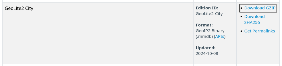
We'll be using an open-source library by MaxMind to query their .mmdb database.
pip install geoip2
Here's a usage example:
import geoip2.database

with geoip2.database.Reader('/path/to/GeoLite2-City.mmdb') as reader:
# or `reader = geoip2.database.Reader('/path/to/GeoLite2-City.mmdb')`

    response = reader.city('203.0.113.0')

    response.country.iso_code
    # 'US'

    response.city.name
    # 'Minneapolis'

    response.postal.code
    # '55455'
Make sure to reuse the reader object wherever possible since its creation is (computationally) expensive.
Enriching WARC with Geolocation Information
The motivation for this exercise is to find the geographical distribution of servers from the response records in the WARC files. We do all the processing on our Spark cluster.
I'll first list out the imports and we can then connect to the Spark Master.
import os
import sys
import shutil
import argparse
from functools import lru_cache

import pandas as pd
from pyspark.sql import Row
from pyspark.sql.functions import pandas_udf
from pyspark.sql import SparkSession, Row
from pyspark.sql.types import (
    StructType,
    StructField,
    StringType,
    IntegerType,
    BooleanType,
    FloatType
)
from warcio import ArchiveIterator
spark = SparkSession.builder \
    .appName("maxmind-warc") \
    .master("spark://spark-master:7077") \
    .getOrCreate()
Now, I'll walk you through our code in a non-sequential manner. You can get the full script at the end.
Extracting IP, URL, and Server from WARC
To extract the desired fields from the WARC files we'll use the warcio library.
First, put the path of the WARC file(s) to process in a text file, say, input.txt.
data_files = spark.sparkContext.textFile("path/to/input.txt")
If there is more than one WARC file path in the .txt file, then Spark creates multiple partitions out of them. We can map a function to these partitions to process them in parallel.
Let's define the functions and the mapping code.
def process_record(record):
    """Return tuple containing ip, url if record is of response type"""
    if record.rec_type == "response":
        ip = record.rec_headers.get_header("WARC-IP-Address", "-")
        url = record.rec_headers.get_header("WARC-Target-URI", "-")
        server = record.http_headers.get_header("Server")
        return (ip, url, server)
    return None

def process_warc(filepath):
    """Read WARC file and yield processed records"""
    with open(filepath, 'rb') as stream:
        for record in ArchiveIterator(stream):
            result = process_record(record)
            if result:
                yield result

def proc_wrapper(_id, iterator):
    """Wrapper function for `process_warc` to handle multiple `warc` files"""
    for filepath in iterator:
        for res in process_warc(filepath):
            yield res
output = data_files.mapPartitionsWithIndex(proc_wrapper)
Here's a breakdown of what is happening here:
proc_wrapperis applied to every partition. Each partition (created from the.txtfile) may contain multiple WARC file paths. So, theproc_wrapperfunction is designed to handle multiple WARC files.process_warcis applied to every WARC file path. In this function, each record in the WARC file is iterated over and is passed toprocess_record.process_recordextracts the record's IP, URL (or hostname), and server fields. The extraction is skipped if the record is not of "response" type.
output contains the RDDs obtained from this processing. We then create a Spark dataframe from this.
warciphost_df = spark.createDataFrame(output, schema=output_schema)
warciphost_df.show()
+---------------+--------------------+
|             ip|            hostname|
+---------------+--------------------+
| 107.163.232.92|http://0.furkid.net/|
|  192.229.64.48|http://01rt.allst...|
|   195.170.8.34|http://0807.syzef...|
| 107.190.226.20|http://0krls.9032...|
| 172.67.142.198|http://101webtemp...|
|   23.108.56.90|http://123any.com...|
| 137.184.244.32|http://137.184.24...|
| 172.67.198.153|http://16trader.c...|
|  220.228.6.123|http://1700866.mk...|
|  220.228.6.241|http://1701057.mw...|
|    220.228.6.6|http://1746747.ut...|
|   61.66.228.75|http://176592.s34...|
|  77.232.40.211|http://2012god.ru...|
|   198.2.232.33|http://201314zz.c...|
|  220.228.6.119|http://2130148.hk...|
| 114.118.10.124|http://21cpm.net/...|
|107.163.236.251|http://25.lasaqls...|
| 208.109.212.43|http://252churcht...|
| 208.109.212.43|http://252churcht...|
|107.163.212.188|http://3.lennonau...|
+---------------+--------------------+
only showing top 20 rows
Adding Geolocation Information
We will use PandasUDF to get geolocation information on the IPs from the MaxMind database.
Similar to a Python UDF, we must define the return datatype here and pass it to the UDF decorator.
But before we do that though, there's a small gotcha here. Any object used in a UDF has to be serializable since the functions are sent over the network as byte streams to be processed on worker nodes. Read more about this problem and how I solved it here:

ip_info_schema = StructType([
    StructField("year", StringType()),
    StructField("postal_code", StringType(), True),
    StructField("latitude", FloatType(), True),
    StructField("longitude", FloatType(), True),
    StructField("accuracy_radius", IntegerType(), True),
    StructField("continent_code", StringType(), True),
    StructField("continent_name", StringType(), True),
    StructField("country_iso_code", StringType(), True),
    StructField("country_name", StringType(), True),
    StructField("subdivision_iso_code", StringType(), True),
    StructField("subdivision_name", StringType(), True),
    StructField("city_name", StringType(), True),
    StructField("metro_code", IntegerType(), True),
    StructField("time_zone", StringType(), True),
])

@pandas_udf(ip_info_schema)
def get_ip_info(ips: pd.Series) -> pd.DataFrame:
    """
    Get reader, query MMDB for info about each IP from a batch of IPs, and return a DataFrame.
    The reader object is created lazily, once per executor.
    Have a look at `SerializableReader` in the `ip_utils` module for more details.
    """
    result = []
    reader = reader_broadcast.value.get_reader()

    for ip in ips:
        try:
            response = reader.city(ip)
            result.append((
                args.year,
                response.postal.code if response else None,
                response.location.latitude if response else None,
                response.location.longitude if response else None,
                response.location.accuracy_radius if response else None,
                response.continent.code if response else None,
                response.continent.name if response else None,
                response.country.iso_code if response else None,
                response.country.name if response else None,
                response.subdivisions[0].iso_code if response and response.subdivisions else None,
                response.subdivisions[0].name if response and response.subdivisions else None,
                response.city.name if response else None,
                response.location.metro_code if response else None,
                response.location.time_zone if response else None,
            ))
        except Exception as e:
            result.append( (args.year, ) + (None,) * (len(ip_info_schema) - 1) )

    return pd.DataFrame(result, columns=ip_info_schema.names)
Here, we have try except to catch exceptions thrown by the MaxMind reader when the IP is not in the database. In such cases, we use None values. We now apply the UDF to the ip column and drop columns where all values are NULL, just in case.
result_df = warciphost_df.withColumn("ip_info", get_ip_info("ip"))
final_df = result_df.select("ip", "host", "server", "ip_info.*").dropna("all")
Getting The Final Dataset Ready
Before we save the final dataset we must first deduplicate the ip column, because there is no use in having redundant information about the same IPs in different rows.
final_df = final_df.dropDuplicates(["ip"])
This dataset's utility is realized when it is combined with other datasets to analyze, say, geographical distributions. So, this step makes sense.
final_df.write.option("delimiter", "\t").mode("append").csv(args.output_dir, header=True)
IPs usually stay in an approximate range for a given region. However, while this is largely true, the inaccuracies can vary depending on the specific IP address and the year in question.
And we have successfully finished the processing! (there's a slight problem with the viewer for the 2024 data, so the 2023 one is linked which was processed identically)
Dataset Statistics
Here are some statistics of the 2024 processed dataset and the code to get that.
from datasets import load_dataset
import plotly.express as px

ds = load_dataset("big-banyan-tree/BBT_CommonCrawl_2024", data_dir="ipmaxmind", split="train")
df = ds.to_pandas()

def plot(x, y, x_label, y_label, title, filename):
    fig = px.bar(
        x=x,
        y=y,
        labels={'x': x_label, 'y': y_label},
        title=title,
        orientation='h'
    )
    fig.write_html(filename, include_plotlyjs="cdn")

server_counts = df.server.value_counts().head(20).sort_values(ascending=True)
continent_counts = df.continent_name.value_counts().head(20).sort_values(ascending=True)
country_counts = df.country_name.value_counts().head(20).sort_values(ascending=True)
city_counts = df.city_name.value_counts().head(20).sort_values(ascending=True)
tz_counts = df.time_zone.value_counts().head(20).sort_values(ascending=True)

plot(server_counts.values, server_counts.index, "Count", "Server Name", "Server Distribution", "server.html")
plot(continent_counts.values, continent_counts.index, "Count", "Continent", "Continent Distribution", "continent.html")
plot(country_counts.values, country_counts.index, "Count", "Country", "Country Distribution", "country.html")
plot(city_counts.values, city_counts.index, "Count", "City", "City Distribution", "city.html")
plot(tz_counts.values, tz_counts.index, "Count", "Time Zone", "Time Zone Distribution", "tz.html")
+----------------------------+--------+
| server                     | count  |
+----------------------------+--------+
| nginx                      | 2379650|
| Apache                     | 2105227|
| cloudflare                 | 1941761|
| LiteSpeed                  | 765267 |
| Microsoft-IIS/10.0         | 269993 |
| Apache/2                   | 120154 |
| nginx/1.18.0 (Ubuntu)      | 117892 |
| imunify360-webshield/1.21  | 115325 |
| openresty                  | 70911  |
| Microsoft-IIS/8.5          | 70556  |
| Apache/2.4.41 (Ubuntu)     | 69965  |
| Apache/2.4.52 (Ubuntu)     | 56484  |
| nginx/1.26.1               | 46348  |
| nginx/1.18.0               | 46221  |
| nginx/1.20.1               | 45859  |
| hcdn                       | 45254  |
| Apache/2.4.29 (Ubuntu)     | 41560  |
| nginx/1.20.2               | 37256  |
| Apache/2.4.61 (Debian)     | 35335  |
| nginx/1.22.1               | 35200  |
+----------------------------+--------+
+---------------+---------+
| continent_name|  count  |
+---------------+---------+
|        Europe | 3907314 |
|  North America| 2646862 |
|           Asia| 1711273 |
|  South America|  149402 |
|       Oceania |   99248 |
|        Africa |   68499 |
|    Antarctica |      44 |
+---------------+---------+
+-----------------+--------+
|   country_name  | count  |
+-----------------+--------+
|  United States  | 2471071|
|      Germany    |  910572|
|       Japan     |  498887|
|      France     |  449864|
|      Russia     |  421970|
| The Netherlands |  306281|
| United Kingdom  |  297906|
|      China      |  252008|
|      Spain      |  184307|
|      Poland     |  183888|
|      Italy      |  179894|
|    Hong Kong    |  165981|
|     Canada      |  158265|
|   Singapore     |  139859|
|      India      |  114508|
|     Czechia     |  104704|
|     Brazil      |   96550|
|    Vietnam      |   95691|
|    Australia    |   89561|
|   South Korea   |   89140|
+-----------------+--------+
+--------------------+--------+
|          city_name | count  |
+--------------------+--------+
|            Ashburn | 348306 |
|        Falkenstein | 213626 |
|          Nuremberg | 146750 |
|          Singapore | 121194 |
|  Frankfurt am Main | 110932 |
|       Los Angeles  | 106062 |
|         Amsterdam  |  97108 |
|              Tokyo |  95188 |
|     St Petersburg  |  92301 |
|           Phoenix  |  83441 |
|         Hong Kong  |  79250 |
|            Dublin  |  78131 |
|            Moscow  |  70383 |
|            London  |  67828 |
|           Helsinki |  65886 |
|            Mumbai  |  64397 |
|             Paris  |  63548 |
|        Strasbourg  |  60291 |
|            Arezzo  |  50888 |
|          Boardman  |  49125 |
+--------------------+--------+
+-----------------------+---------+
| time_zone             | count   |
+-----------------------+---------+
| America/Chicago       | 1249152 |
| Europe/Berlin         |  910572 |
| America/New_York      |  728243 |
| Asia/Tokyo            |  498887 |
| Europe/Paris          |  449864 |
| Europe/Moscow         |  413199 |
| America/Los_Angeles   |  366192 |
| Europe/Amsterdam      |  306281 |
| Europe/London         |  297906 |
| Asia/Shanghai         |  252008 |
| Europe/Warsaw         |  183888 |
| Europe/Madrid         |  183483 |
| Europe/Rome           |  179894 |
| Asia/Hong_Kong        |  165981 |
| America/Toronto       |  145653 |
| Asia/Singapore        |  139859 |
| Asia/Kolkata          |  114508 |
| Asia/Bangkok          |  113994 |
| Europe/Prague         |  104704 |
| America/Phoenix       |   94997 |
+-----------------------+---------+
Open Sourcing our Dataset
The dataset used in this analysis is fully open-sourced by us and is available on HuggingFace 🤗 for download. We encourage you to tinker with the dataset and can't wait to see what you build with it!

Our dataset has two parts (separated as directories on HF):
- ipmaxmind_out
- script_extraction_out
"ipmaxmind_out", as you saw in this blog, has IPs from response records of the WARC files enriched with information from MaxMind's database.
"script_extraction_out" has IP, server among other columns, and the src attributes of the HTML content in the WARC response records. Visit the datasets' HuggingFace repositories for more information.